Chapter 3: Classical search algorithms
DIT411/TIN175, Artificial Intelligence
Peter Ljunglöf
19 January, 2018
Deadline for forming groups
-
Today is the deadline for forming groups.
- if you have any problems, please talk to me in the break
- e.g., if you cannot contact one of your group members
- or if you don’t have a group yet
-
Don’t forget to create a Github team and clone the Shrdlite repository
- then email me with information about your group
-
Today we will decide your exact supervision time and your supervisor
Table of contents
- Introduction (R&N 3.1–3.3)
- Graphs and searching
- Example problems
- A generic searching algorithm
- Graphs and searching
- State-space search: Complexity dimensions
- Directed Graphs
- Example: Travel in Romania
- Example: Grid game
- Example: Vacuum-cleaning agent
- Example: The 8-puzzle
- Example: The 8-queens problem
- Example: The 8-queens problem (alternative)
- Example: Knuth’s conjecture
- Example: Robotic assembly
- How do we search in a graph?
- Illustration of generic search
- A generic tree search algorithm
- Using tree search on a graph
- Turning tree search into graph search
- Tree search vs. graph search
- Graph nodes vs. search nodes
- Uninformed search (R&N 3.4)
- Heuristic search (R&N 3.5–3.6)
- Greedy best-first search
- A* search
- Admissible and consistent heuristics
- Heuristic search
- Greedy best-first search
- Greedy search example: Romania
- Greedy search is not optimal
- Best-first search and infinite loops
- Complexity of Best-first Search
- A* search
- A* search
- Complexity of A* search
- A* search example: Romania
- A* search is optimal
- A* always finds a solution
- Admissibility (optimality) of A*
- Why is A* optimal?
- Illustration: Why is A* optimal?
- Question time: Heuristics for the 8 puzzle
- Dominating heuristics
- Heuristics from a relaxed problem
- Summary of tree search strategies
- Example demo
Introduction (R&N 3.1–3.3)
Graphs and searching
Example problems
A generic searching algorithm
Graphs and searching
-
Often we are not given an algorithm to solve a problem, but only
a specification of a solution — we have to search for it. -
A typical problem is when the agent is in one state, it has a set of
deterministic actions it can carry out, and wants to get to a goal state. -
Many AI problems can be abstracted into the problem of finding
a path in a directed graph. -
Often there is more than one way to represent a problem as a graph.
State-space search: Complexity dimensions
| Observable? | fully |
| Deterministic? | deterministic |
| Episodic? | episodic |
| Static? | static |
| Discrete? | discrete |
| N:o of agents | single |
Most complex problems (partly observable, stochastic, sequential)
usualy have components using state-space search.
Directed Graphs
-
A graph consists of a set \(N\) of nodes and a set \(A\) of ordered pairs of nodes,
called arcs or edges.-
Node \(n_2\) is a neighbor of \(n_1\) if there is an arc from \(n_1\) to \(n_2\).
That is, if \( (n_1, n_2) \in A \). -
A path is a sequence of nodes \( (n_0, n_1, \ldots, n_k) \) such that \( (n_{i-1}, n_i) \in A \).
-
The length of path \( (n_0, n_1, \ldots, n_k) \) is \(k\).
-
A solution is a path from a start node to a goal node,
given a set of start nodes and goal nodes. -
(Russel & Norvig sometimes call the graph nodes states).
-
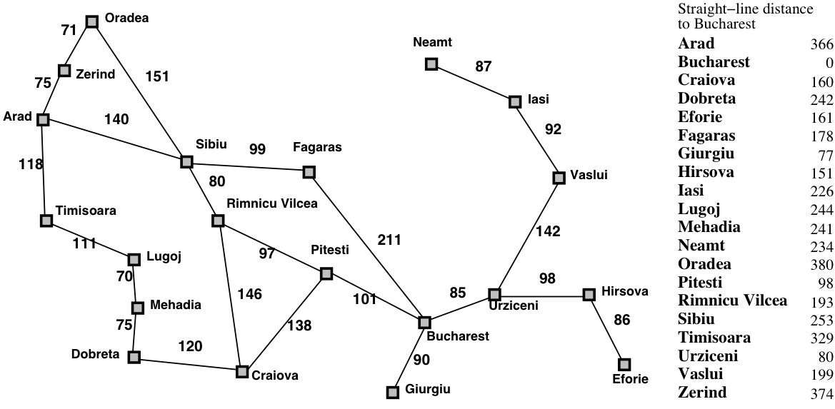
Example: Travel in Romania
We want to drive from Arad to Bucharest in Romania

Example: Grid game
Grid game: Rob needs to collect coins
\( C_{1}, C_{2}, C_{3}, C_{4} \),
without running out of fuel, and end up at location (1,1):
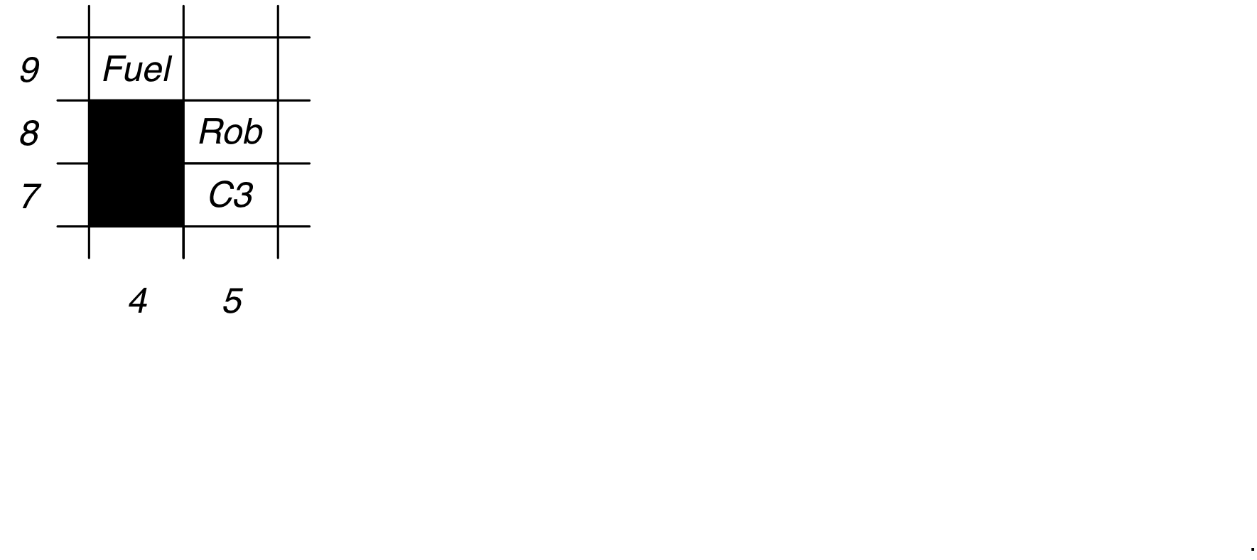
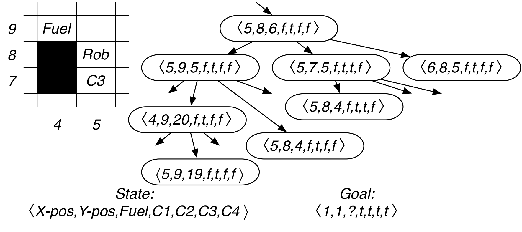
What is a good representation of the search states and the goal?
Example: Vacuum-cleaning agent
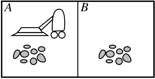
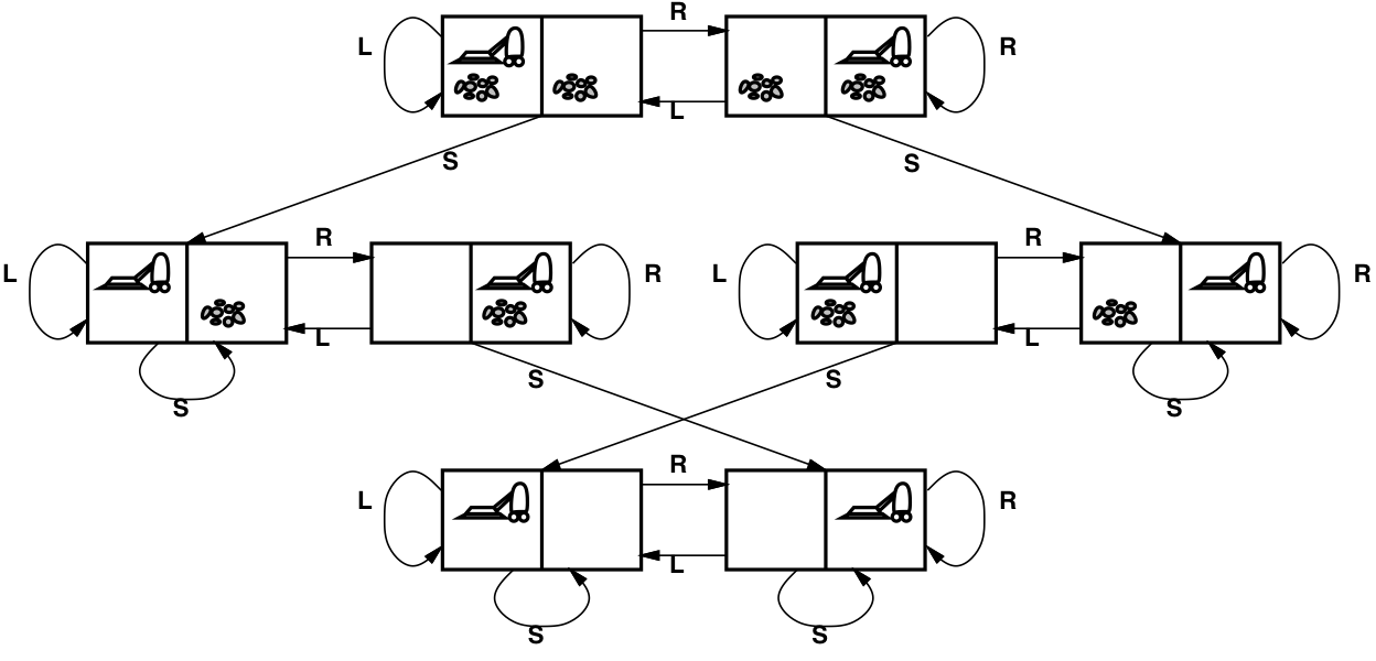
| States | [room A dirty?, room B dirty?, robot location] |
| Initial state | any state |
| Actions | left, right, suck, do-nothing |
| Goal test | [false, false, –] |
Example: The 8-puzzle
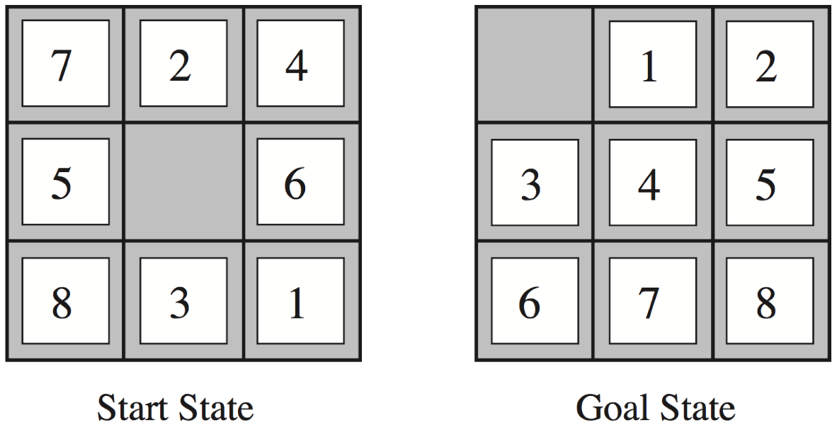
| States | a 3 x 3 matrix of integers |
| Initial state | any state |
| Actions | move the blank space: left, right, up, down |
| Goal test | equal to the goal state |
Example: The 8-queens problem
| States | any arrangement of 0 to 8 queens on the board |
| Initial state | no queens on the board |
| Actions | add a queen to any empty square |
| Goal test | 8 queens on the board, none attacked |
This gives us \( 64 \times 63 \times\cdots\times 57 \approx 1.8\times10^{14} \) possible paths to explore!
Example: The 8-queens problem (alternative)
| States | one queen per column in leftmost columns, none attacked |
| Initial state | no queens on the board |
| Actions | add a queen to a square in the leftmost empty column, make sure that no queen is attacked |
| Goal test | 8 queens on the board, none attacked |
Using this formulation, we have only 2,057 paths!
Example: Knuth’s conjecture
Donald Knuth conjectured that all positive integers can be obtained by starting with
the number 4 and applying some combination of the factorial, square root, and floor.
\[ \left\lfloor \sqrt{\sqrt{\sqrt{\sqrt{\sqrt{(4!)!}}}}}\right\rfloor = 5 \]
| States | algebraic numbers \( (1, 2.5, 9, \sqrt{2}, 1.23\cdot 10^{456}, \sqrt{\sqrt{2}}, \ldots) \) |
| Initial state | 4 |
| Actions | apply factorial, square root, or floor operation |
| Goal test | a given positive integer (e.g., 5) |
Example: Robotic assembly
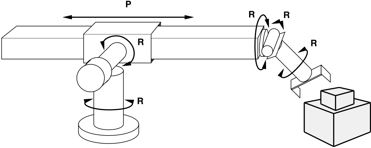
| States | real-valued coordinates of robot joint angles parts of the object to be assembled |
| Actions | continuous motions of robot joints |
| Goal test | complete assembly of the object |
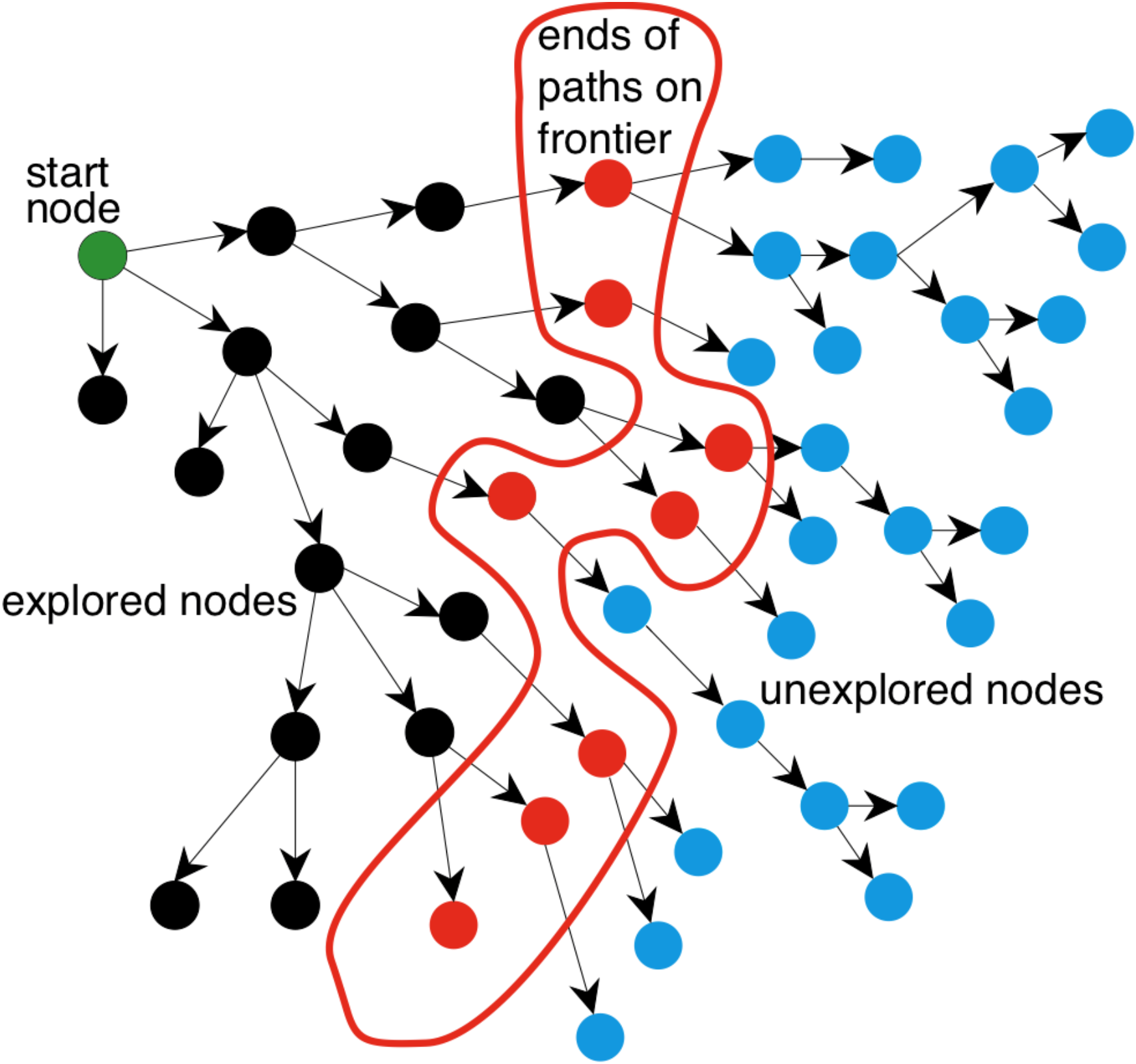
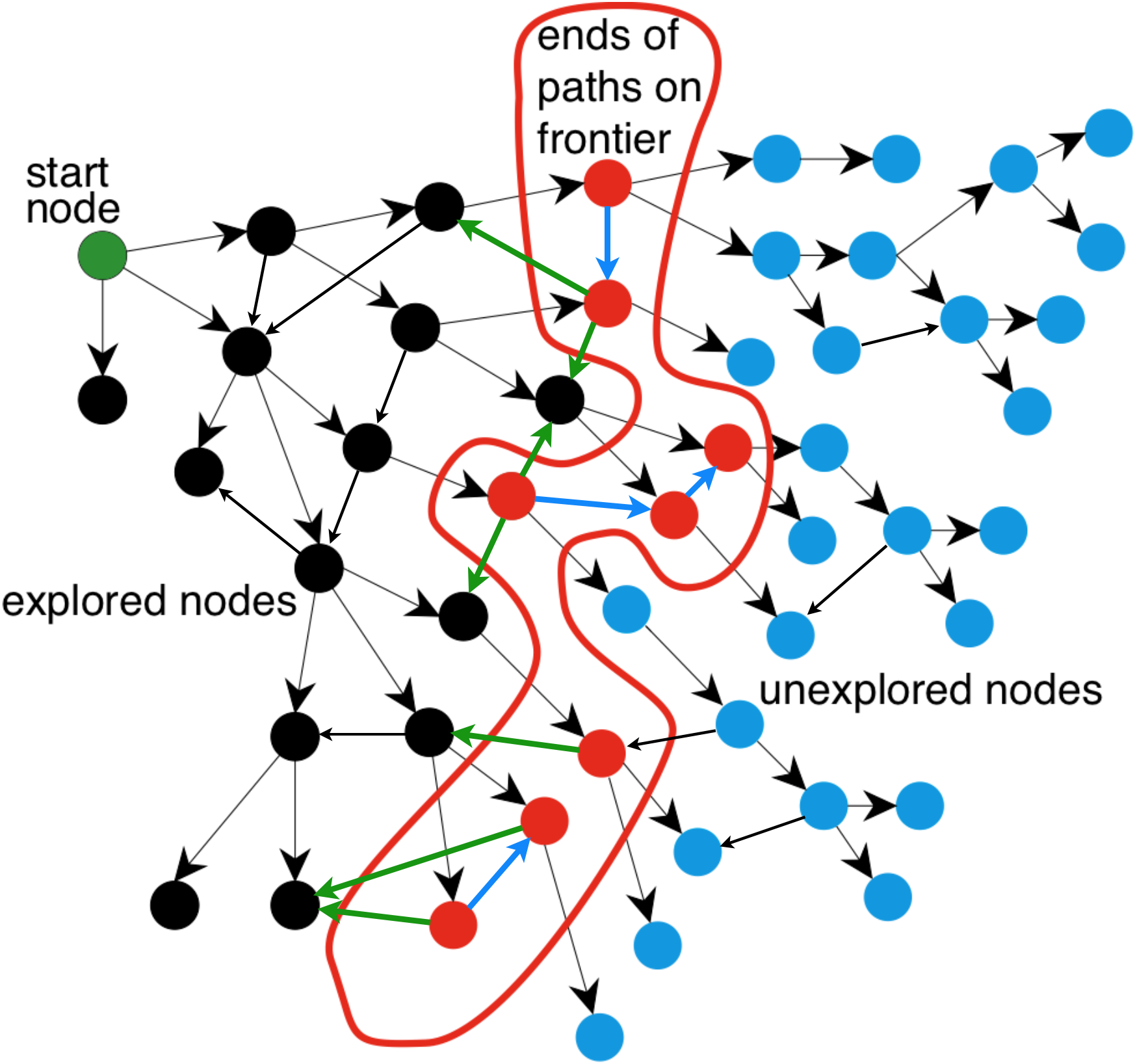
How do we search in a graph?
-
A generic search algorithm:
-
Given a graph, start nodes, and a goal description, incrementally
explore paths from the start nodes. -
Maintain a frontier of nodes that are to be explored.
-
As search proceeds, the frontier expands into the unexplored nodes
until a goal node is encountered. -
The way in which the frontier is expanded defines the search strategy.
-
Illustration of generic search
A generic tree search algorithm
- Tree search: Don’t check if nodes are visited multiple times
- function Search(graph, initialState, goalState):
- initialise frontier using the initialState
- while frontier is not empty:
- select and remove node from frontier
- if node.state is a goalState then return node
- for each child in ExpandChildNodes(node, graph):
- add child to frontier if child is not in frontier or exploredSet
- return failure
Using tree search on a graph
-
- explored nodes might be revisited
- frontier nodes might be duplicated
Turning tree search into graph search
- Graph search: Keep track of visited nodes
- function Search(graph, initialState, goalState):
- initialise frontier using the initialState
- initialise exploredSet to the empty set
- while frontier is not empty:
- select and remove node from frontier
- if node.state is a goalState then return node
- add node to exploredSet
- for each child in ExpandChildNodes(node, graph):
- add child to frontier if child is not in frontier or exploredSet
- return failure
Tree search vs. graph search
-
Tree search
- Pro: uses less memory
- Con: might visit the same node several times
-
Graph search
- Pro: only visits nodes at most once
- Con: uses more memory
-
Note: The pseudocode in these slides (and the course book)
is not the only possible! E.g., Wikipedia uses a different variant.
Graph nodes vs. search nodes
- Search nodes are not the same as graph nodes!
- Search nodes should contain more information:
- the corresponding graph node (called state in R&N)
- the total path cost from the start node
- the estimated (heuristic) cost to the goal
- enough information to be able to calculate the final path
- procedure ExpandChildNodes(parent, graph):
- for each (action, child, edgecost) in graph.successors(parent.state):
- yield new SearchNode(child,
- …total cost so far…,
- …estimated cost to goal…,
- …information for calculating final path…)
- yield new SearchNode(child,
- for each (action, child, edgecost) in graph.successors(parent.state):
Uninformed search (R&N 3.4)
Depth-first search
Breadth-first search
Uniform-cost search
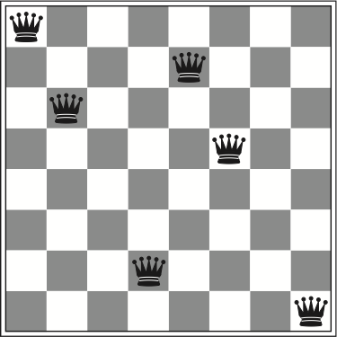
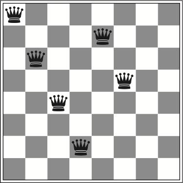
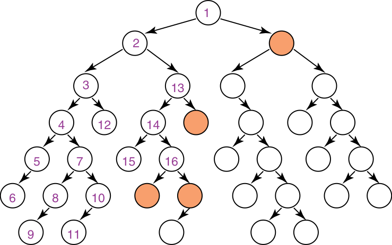
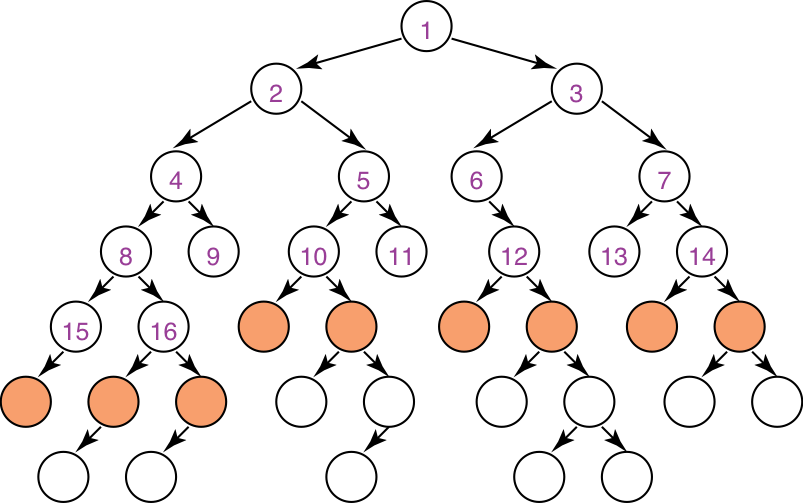
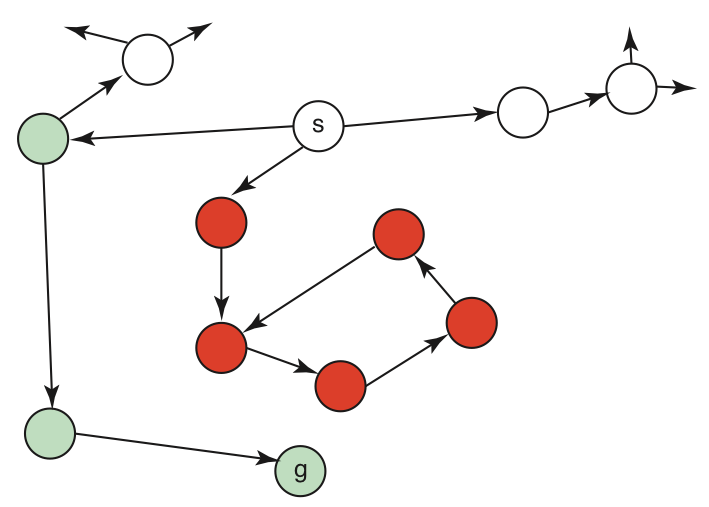
Question time: Depth-first search
Which shaded goal will a depth-first search find first?
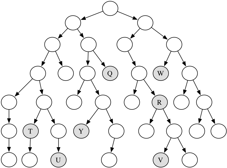
Question time: Breadth-first search
Which shaded goal will a breadth-first search find first?
Depth-first search
-
Depth-first search treats the frontier as a stack.
-
It always selects one of the last elements added to the frontier.
-
If the list of nodes on the frontier is \( [p_{1},p_{2},p_{3},\ldots] \), then:
- \( p_{1} \) is selected (and removed).
- Nodes that extend \( p_{1} \) are added to the front of the stack (in front of \( p_{2} \)).
- \( p_{2} \) is only selected when all nodes from \( p_{1} \) have been explored.
Illustrative graph: Depth-first search
Complexity of depth-first search
-
Does DFS guarantee to find the path with fewest arcs?
-
What happens on infinite graphs or on graphs with cycles if there is a solution?
-
What is the time complexity as a function of the path length?
-
What is the space complexity as a function of the path length?
-
How does the goal affect the search?
Breadth-first search
-
Breadth-first search treats the frontier as a queue.
-
It always selects one of the earliest elements added to the frontier.
-
If the list of paths on the frontier is \( [p_{1},p_{2},\ldots,p_{r}] \), then:
- \( p_{1} \) is selected (and removed).
- Its neighbors are added to the end of the queue, after \( p_{r} \).
- \( p_{2} \) is selected next.
Illustrative graph: breadth-first search
Complexity of breadth-first search
-
Does BFS guarantee to find the path with fewest arcs?
-
What happens on infinite graphs or on graphs with cycles if there is a solution?
-
What is the time complexity as a function of the path length?
-
What is the space complexity as a function of the path length?
-
How does the goal affect the search?
Uniform-cost search
- Weighted graphs:
- Sometimes there are costs associated with arcs.
The cost of a path is the sum of the costs of its arcs. \[ cost(n_{0},\dots,n_{k}) = \sum_{i=1}^{k}\left|(n_{i-1},n_{i})\right| \] An optimal solution is one with minimum cost.
- Sometimes there are costs associated with arcs.
- Uniform-cost search (aka Lowest-cost-first search):
- Uniform-cost search selects a path on the frontier with the lowest cost.
- The frontier is a priority queue ordered by path cost.
- It finds a least-cost path to a goal node — i.e., uniform-cost search is optimal
- When arc costs are equal \(\Rightarrow\) breadth-first search.
Heuristic search (R&N 3.5–3.6)
Greedy best-first search
A* search
Admissible and consistent heuristics
Heuristic search
- Previous methods don’t use the goal to select a path to explore.
-
Main idea: don’t ignore the goal when selecting paths.
-
Often there is extra knowledge that can guide the search: heuristics.
-
\( h(n) \) is an estimate of the cost of the shortest path from node \(n\)
to a goal node. -
\(h(n)\) needs to be efficient to compute.
-
\(h(n)\) is an underestimate if there is no path from \(n\) to a goal
with cost less than \(h(n)\). -
An admissible heuristic is a nonnegative underestimating heuristic function:
\( 0 \leq h(n) \leq cost(\textit{best path from n to goal}) \)
-
Example heuristic functions
-
Here are some example heuristic functions:
-
If the nodes are points on a Euclidean plane and the cost is the distance,
\(h(n)\) can be the straight-line distance (SLD) from \(n\) to the closest goal. -
If the nodes are locations and cost is time, we can use the distance to
a goal divided by the maximum speed, \(h(n)=d(n)/v_{\max}\)
(or the average speed, \(h(n)=d(n)/v_{\textrm{avg}}\), which makes it non-admissible). -
If the graph is a 2D grid maze, then we can use the Manhattan distance.
-
If the goal is to collect all of the coins and not run out of fuel, we can
use an estimate of how many steps it will take to collect the coins
and return to goal position, without caring about the fuel consumption.
-
-
A heuristic function can be found by solving a simpler (less constrained)
version of the problem.
Example heuristic: Romania distances
Greedy best-first search
-
Main idea: select the path whose end is closest to a goal
according to the heuristic function. -
Best-first search selects a path on the frontier with minimal \(h\)-value.
-
It treats the frontier as a priority queue ordered by \(h\).
Greedy search example: Romania
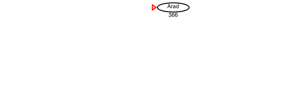
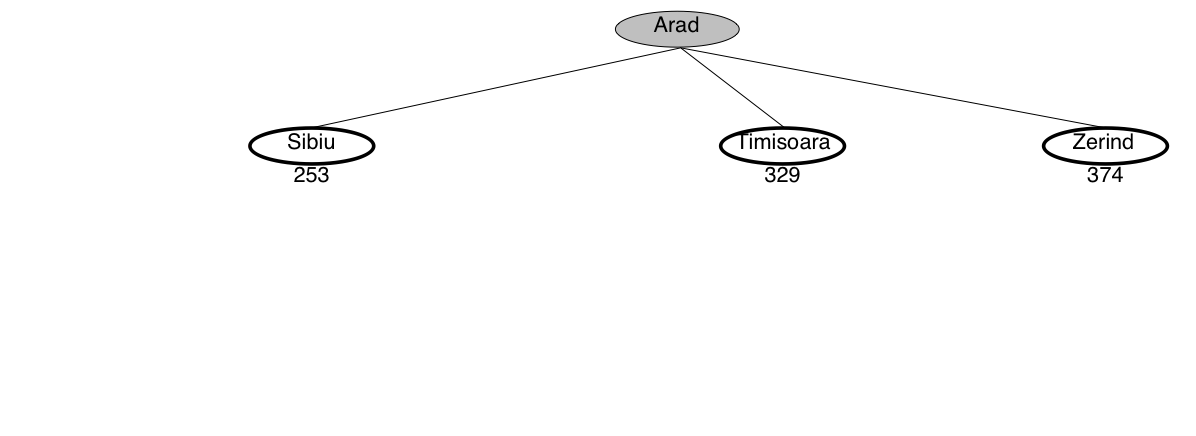
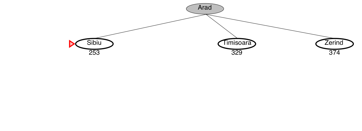
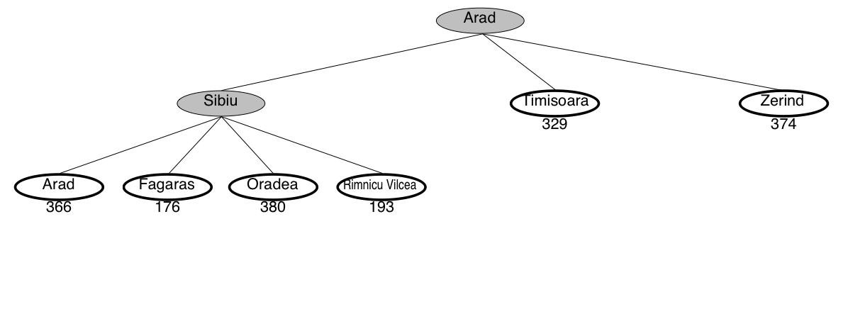
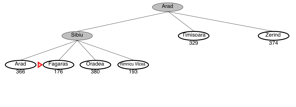
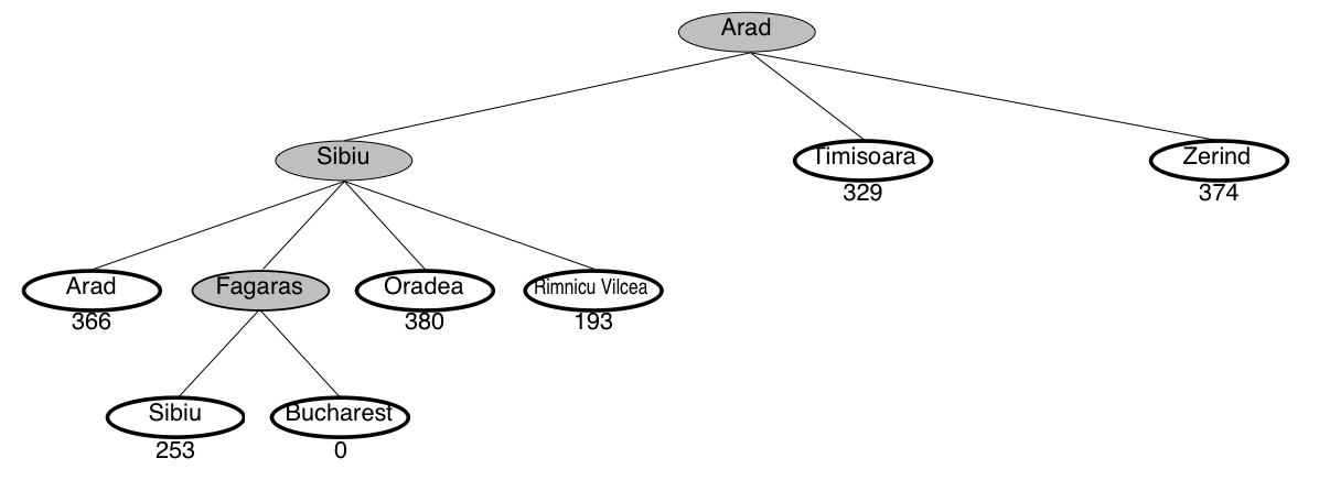
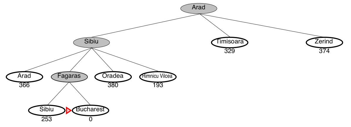
This is not the shortest path!
Greedy search is not optimal
- Greedy search returns the path: Arad–Sibiu–Fagaras–Bucharest (450km)
- The optimal path is: Arad–Sibiu–Rimnicu–Pitesti–Bucharest (418km)

Best-first search and infinite loops
Best-first search might fall into an infinite loop!
Complexity of Best-first Search
-
Does best-first search guarantee to find the path with fewest arcs?
-
What happens on infinite graphs or on graphs with cycles if there is a solution?
-
What is the time complexity as a function of the path length?
-
What is the space complexity as a function of the path length?
-
How does the goal affect the search?
A* search
-
A* search uses both path cost and heuristic values.
-
\(cost(p)\) is the cost of path \(p\).
-
\(h(p)\) estimates the cost from the end node of \(p\) to a goal.
-
\(f(p) = cost(p)+h(p)\), estimates the total path cost
of going from the start node, via path \(p\) to a goal:\[ \underbrace{ \underbrace{start\xrightarrow{\textrm{path}~p}~}_{cost(p)} n \underbrace{~\xrightarrow{\textrm{estimate}}~goal}_{h(p)} }_{f(p)} \]
A* search
-
A* is a mix of uniform-cost search and best-first search.
-
It treats the frontier as a priority queue ordered by \(f(p)\).
-
It always selects the node on the frontier with
the lowest estimated distance from the start
to a goal node constrained to go via that node.
Complexity of A* search
-
Does A* search guarantee to find the path with fewest arcs?
-
What happens on infinite graphs or on graphs with cycles if there is a solution?
-
What is the time complexity as a function of the path length?
-
What is the space complexity as a function of the path length?
-
How does the goal affect the search?
A* search example: Romania
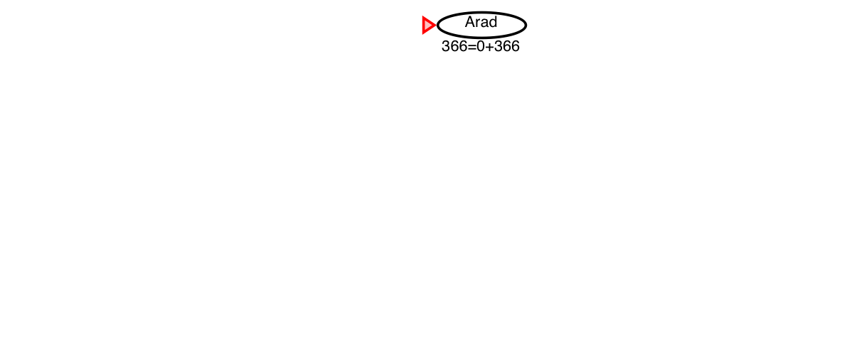
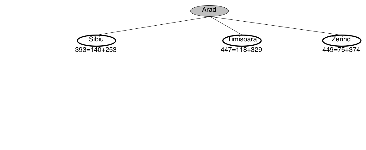
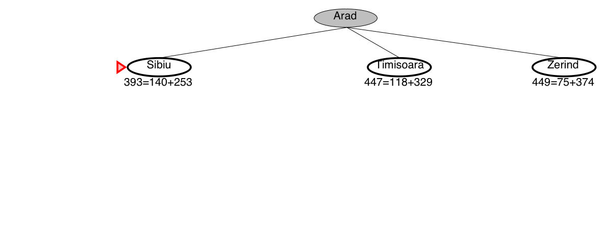
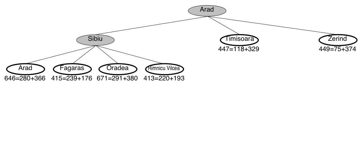
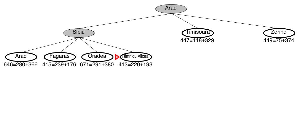
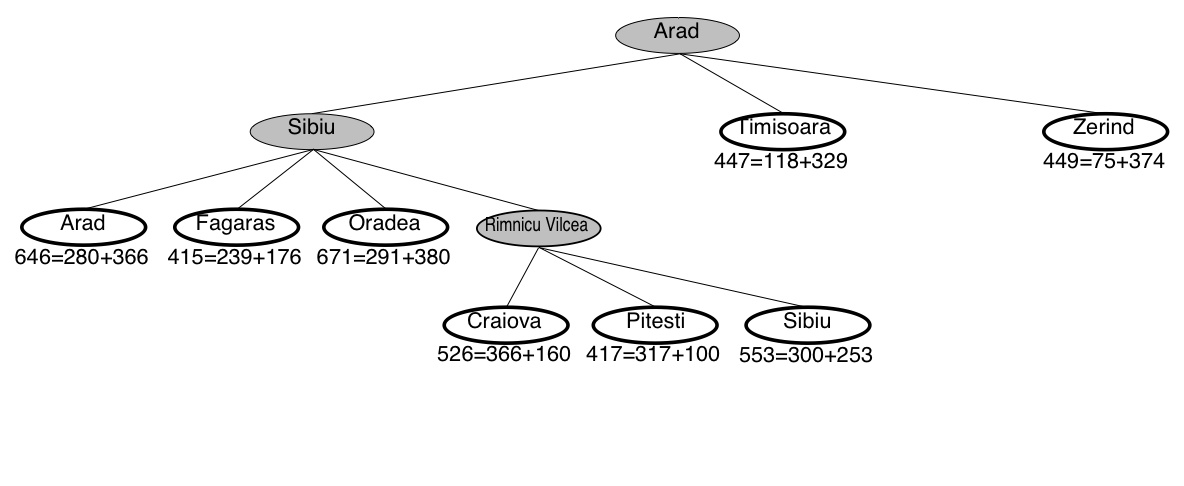
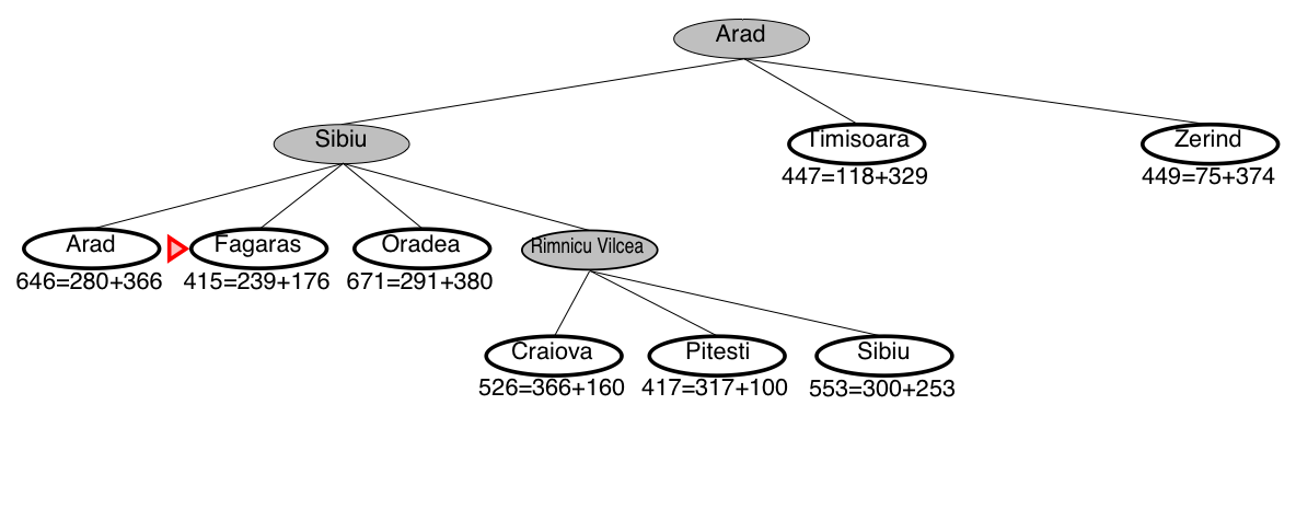
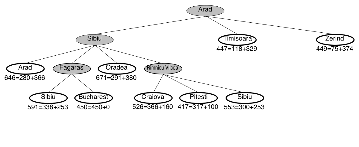
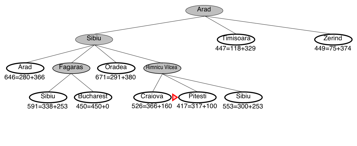
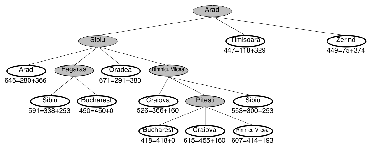
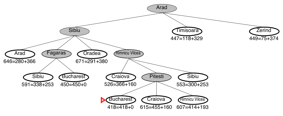
A* guarantees that this is the shortest path!
Note that we didn’t stop when we added Bucharest to the frontier.
Instead, we stopped when we removed Bucharest from the frontier!
A* search is optimal
- The optimal path is: Arad–Sibiu–Rimnicu–Pitesti–Bucharest (418km)
A* always finds a solution
-
A* will always find a solution if there is one, because:
-
The frontier always contains the initial part of a path to a goal,
before that goal is selected. -
A* halts, because the costs of the paths on the frontier keeps increasing,
and will eventually exceed any finite number.
-
Admissibility (optimality) of A*
-
If there is a solution, A* always finds an optimal one first, provided that:
-
the branching factor is finite,
-
arc costs are bounded above zero
(i.e., there is some \(\epsilon>0\) such that all
of the arc costs are greater than \(\epsilon\)), and -
\(h(n)\) is nonnegative and an underestimate of
the cost of the shortest path from \(n\) to a goal node.
-
-
These requirements ensure that \(f\) keeps increasing.
Why is A* optimal?
-
The \(f\) values in A* are increasing, therefore:
first A* expands all nodes with \( f(n) < C \) then A* expands all nodes with \( f(n) = C \) finally A* expands all nodes with \( f(n) > C \) -
A* will not expand any nodes with \( f(n) > C* \),
where \(C*\) is the cost of an optimal solution. -
(Note: all this assumes that the heuristics is admissible)
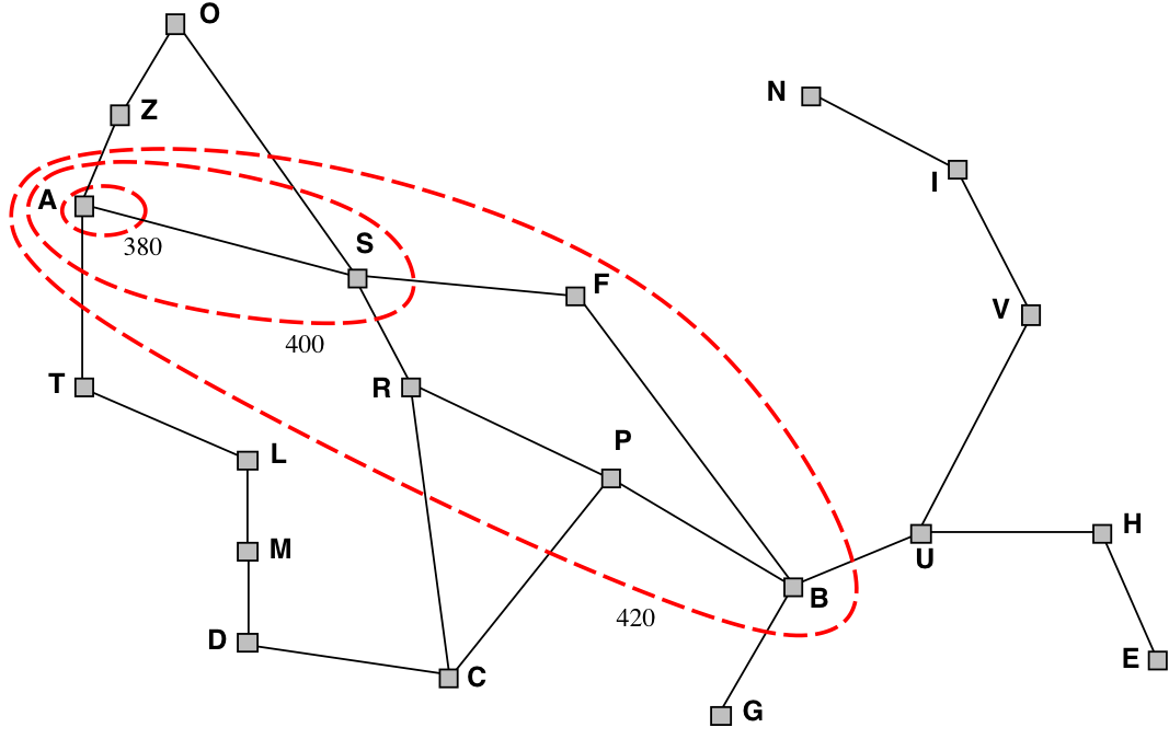
Illustration: Why is A* optimal?
-
A* gradually adds “\(f\)-contours” of nodes (cf. BFS adds layers)
-
Contour \(i\) has all nodes with \(f=f_{i}\), where \(f_{i}<f_{i+1}\)
Question time: Heuristics for the 8 puzzle
- \(h_{1}(n)\) = number of misplaced tiles
- \(h_{2}(n)\) = total Manhattan distance
(i.e., no. of squares from desired location of each tile)
- \(h_{1}(StartState)\) = 8
- \(h_{2}(StartState)\) = 3+1+2+2+2+3+3+2 = 18
Dominating heuristics
-
If (admissible) \(h_{2}(n)\geq h_{1}(n)\) for all \(n\),
then \(h_{2}\) dominates \(h_{1}\) and is better for search. -
Typical search costs (for 8-puzzle):
depth = 14 DFS ≈ 3,000,000 nodes
A*(\(h_1\)) = 539 nodes
A*(\(h_2\)) = 113 nodesdepth = 24 DFS ≈ 54,000,000,000 nodes
A*(\(h_1\)) = 39,135 nodes
A*(\(h_2\)) = 1,641 nodes -
Given any admissible heuristics \(h_{a}\), \(h_{b}\), the maximum heuristics \(h(n)\)
is also admissible and dominates both: \[ h(n) = \max(h_{a}(n),h_{b}(n)) \]
Heuristics from a relaxed problem
-
Admissible heuristics can be derived from the exact solution cost of
a relaxed problem:-
If the rules of the 8-puzzle are relaxed so that a tile can move anywhere,
then \(h_{1}(n)\) gives the shortest solution -
If the rules are relaxed so that a tile can move to any adjacent square,
then \(h_{2}(n)\) gives the shortest solution
-
-
Key point: the optimal solution cost of a relaxed problem is
never greater than the optimal solution cost of the real problem
Summary of tree search strategies
| Search strategy |
Frontier selection | Halts if solution? | Halts if no solution? | Space usage |
|---|---|---|---|---|
| Depth first | Last node added | No | No | Linear |
| Breadth first | First node added | Yes | No | Exp |
| Best first | Minimal \(h(p)\) | No | No | Exp |
| Uniform cost | Minimal \(cost(p)\) | Yes | No | Exp |
| A* | \(f(n)=g(n)+h(n)\) | Yes | No | Exp |
- Halts if: If there is a path to a goal, it can find one, even on infinite graphs.
- Halts if no: Even if there is no solution, it will halt on a finite graph (with cycles).
- Space: Space complexity as a function of the length of the current path.
Example demo
-
Here is an example demo of several different search algorithms,
including A*. And you can play with different heuristics: -
Note that this demo is tailor-made for planar grids,
which is a special case of all possible search graphs.- (e.g., the Shrdlite graph will not be a planar grid)