Chapter 7: Constraint satisfaction problems
DIT411/TIN175, Artificial Intelligence
Peter Ljunglöf
30 January, 2018
Table of contents
CSP: Constraint satisfaction problems (R&N 7.1)
Formulating a CSP
Constraint graph
Constraint satisfaction problems (CSP)
-
Standard search problem:
- the state is a “black box”, any data structure that supports:
- goal test, cost evaluation, successor
- the state is a “black box”, any data structure that supports:
-
CSP is a more specific search problem:
-
the state is defined by variables \(X_{i}\), taking values from the domain \(\mathbf{D}_{i}\)
-
the goal test is a set of constraints specifying allowable combinations
of values for subsets of variables
-
-
Since CSP is more specific, it allows useful algorithms with more power than standard search algorithms
States and variables
Just a few variables can describe many states:
| \(n\) | binary variables can describe | \(2^{n}\) states |
|---|---|---|
| 10 | binary variables can describe | \(2^{10}\) = 1,024 |
| 20 | binary variables can describe | \(2^{20}\) = 1,048,576 |
| 30 | binary variables can describe | \(2^{30}\) = 1,073,741,824 |
| 100 | binary variables can describe | \(2^{100}\) = 1,267,650,600,228,229, 401,496,703,205,376 |
Hard and soft constraints
-
Given a set of variables, assign a value to each variable that either
- satisfies some set of constraints:
- satisfiability problems — “hard constraints”
- satisfies some set of constraints:
-
- or minimizes some cost function,
where each assignment of values to variables has some cost:- optimization problems — “soft constraints” — “preferences”
- or minimizes some cost function,
-
- many problems are a mix of hard constraints and preferences:
- constraint optimization problems
- many problems are a mix of hard constraints and preferences:
- In this course we will focus on satisfiability problems
Relationship to search
-
Differences between CSP and general search problems:
-
The path to a goal isn’t important, only the solution is.
-
There are no predefined starting nodes.
-
Often these problems are huge, with thousands of variables,
so systematically searching the space is infeasible. -
For optimization problems, there are no well-defined goal nodes.
-
Formulating a CSP
-
A CSP is characterized by
-
A set of variables \(X_{1},X_{2},\ldots,X_{n}\).
-
Each variable \(X_{i}\) has an associated domain \(\mathbf{D}_{i}\) of possible values.
-
There are hard constraints \(C_{X_i,\ldots,X_j}\) on various subsets of the variables
which specify legal combinations of values for these variables. -
A solution to the CSP is an assignment of a value to each variable
that satisfies all the constraints.
-
Example: Scheduling activities
| Variables: | \(A, B, C, D, E\) representing starting times of various activities. (e.g., courses and their study periods) |
| Domains: | \(\mathbf{D}_{A}=\mathbf{D}_{B}=\mathbf{D}_{C}=\mathbf{D}_{D}=\mathbf{D}_{E}=\{1,2,3,4\}\) |
| Constraints: | \((B\neq3), (C\neq2), (A\neq B), (B\neq C), (C<D), (A=D),\) \((E<A), (E<B), (E<C), (E<D), (B\neq D)\) |
Example: Crossword puzzle
-
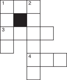
-
Words: ant, big, bus, car, has, book, buys, hold, lane, year, beast, ginger, search, symbol, syntax, …
Dual representations
Many problems can be represented in different ways as a CSP, e.g., the crossword puzzle:
-
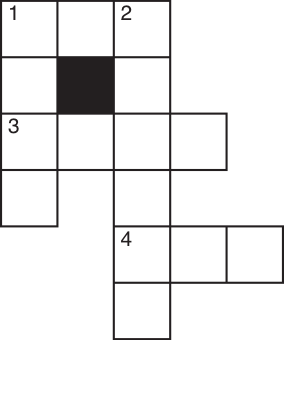
- One representation:
- each variable represent one word
- the domain is all words in the lexicon
- constraints specify that the letters
on the intersections must be the same - 5 variables, 5 constraints, \(|\mathbf{D}|\) ≈ 100,000
- Dual representation:
- each variable represent an individual square
- the domain is the letters in the alphabet
- constraints specify that letter combinations must
be in the lexicon - 15 variables, 5 constraints, \(|\mathbf{D}|\) = 26
Example: Map colouring
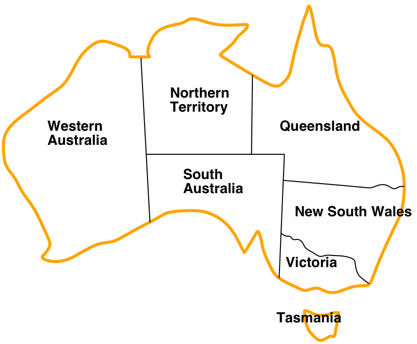
| Variables: | \(\mathit{WA}, NT, Q, \mathit{NSW}, V, \mathit{SA}, T\) |
| Domains: | \(\mathbf{D}_{i}=\{red,green,blue\}\) |
| Constraints: | adjacent regions must have different colors, i.e., \(\mathit{WA}\neq NT,\mathit{WA}\neq\mathit{SA},NT\neq\mathit{SA},NT\neq Q,\ldots\) |
Example: Map colouring
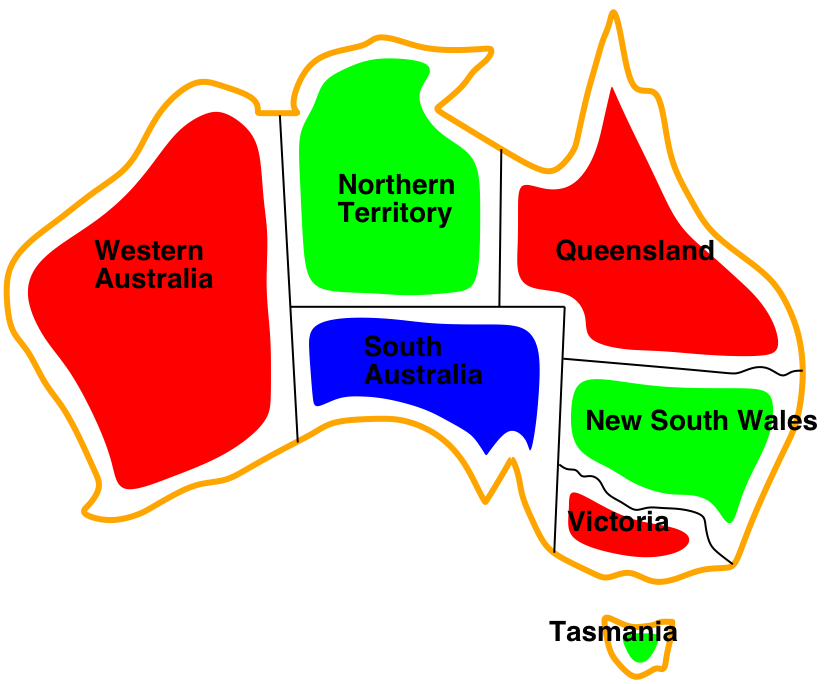
- Solutions are assignments satisfying all constraints, e.g.,
\(\{\mathit{WA}=red,NT=green,Q=red,\mathit{NSW}=green,\)
\(V=red,\mathit{SA}=blue,T=green\}\)
Constraint graph
-
Binary CSP: each constraint relates at most two variables
(note: this does not say anything about the domains) -
Constraint graph: every variable is a node, every binary constraint is an arc
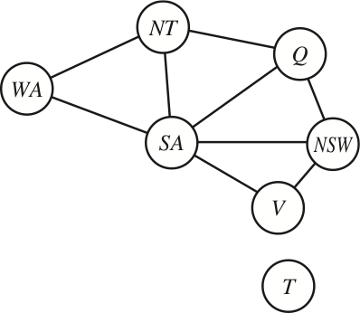
- CSP algorithms can use the graph structure to speed up search,
e.g., Tasmania is an independent subproblem.
Example: Cryptarithmetic puzzle
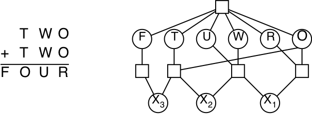
| Variables: | \(F,T,U,W,R,O,X_{1},X_{2},X_{3}\) |
| Domains: | \(\{0,1,2,3,4,5,6,7,8,9\}\) |
| Constraints: | \(\mathit{Alldiff}(F,T,U,W,R,O)\), \(O+O=R+10\cdot X_{1}\), etc. |
| Note: | This is not a binary CSP! The graph is a constraint hypergraph |
Example: Sudoku
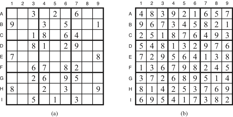
| Variables: | \(A_1\ldots A_9,B_1,\ldots,E_5,\ldots,I_9\) |
| Domains: | \(\{1,2,3,4,5,6,7,8,9\}\) |
| Constraints: | \(\mathit{Alldiff}(A_1,\ldots,A_9)\), …, \(\mathit{Alldiff}(A_5,\ldots,I_5)\), …, \(\mathit{Alldiff}(D_1,\ldots,F_3)\), …, \(B_1=9\), …, \(F_6=8\), …, \(I_7=3\) |
Example: n-queens
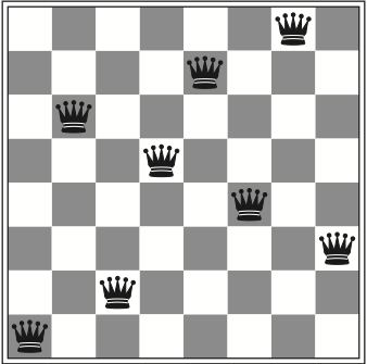
| Variables: | \(Q_1, Q_2,\ldots, Q_n\) |
| Domains: | \(\{1,2,3,\ldots,n\}\) |
| Constraints: | \(\mathit{Alldiff}(Q_1,Q_2,\ldots,Q_n)\), \(Q_i-Q_j \neq |i-j|\) (\(1\leq i<j\leq n\)) |
CSP Varieties
- Discrete variables, finite domains:
- \(n\) variables, domain size \(d\) \(\Rightarrow\) \(O(d^{n})\) complete assignments
- this is what we discuss in this course
- Discrete variables, infinite domains (integers, strings, etc.)
- e.g., job scheduling — variables are start/end times for each job
- we need a constraint language for formulating the constraints
(e.g., \(T_{1}+d_1\leq T_{2}\)) - linear constraints are solvable — nonlinear are undecidable
- Continuous variables:
- e.g., scheduling for Hubble Telescope observations and manouvers
- linear constraints (linear programming) — solvable in polynomial time!
Different kinds of constraints
- Unary constraints involve a single variable:
- e.g., \(SA\neq green\)
- Binary constraints involve pairs of variables:
- e.g., \(SA\neq WA\)
- Global constraints (or higher-order) involve 3 or more variables:
- e.g., \(\mathit{Alldiff}(WA,NT,SA)\)
- all global constraints can be reduced to a number of binary constraints
(but this might lead to an explosion of the number of constraints)
- Preferences (or soft constraints):
- “constraint optimization problems”
- often representable by a cost for each variable assignment
- not discussed in this course
CSP as a search problem (R&N 7.3–7.3.2)
Backtracking search
Heuristics: Improving backtracking efficiency
Generate-and-test algorithm
-
Generate the assignment space \(\mathbf{D} = \mathbf{D}_{V_{1}}\times\mathbf{D}_{V_{2}}\times\cdots\times\mathbf{D}_{V_{n}}\)
Test each assignment with the constraints. -
Example:
\(\mathbf{D}\) = \(\mathbf{D}_{A}\times\mathbf{D}_{B}\times\mathbf{D}_{C}\times\mathbf{D}_{D}\times\mathbf{D}_{E}\) = \(\{1,2,3,4\}\times\cdots\times\{1,2,3,4\}\) = \(\{(1,1,1,1,1),(1,1,1,1,2),\ldots,(4,4,4,4,4)\}\) -
How many assignments need to be tested for \(n\) variables,
each with domain size \(d=|\mathbf{D_i}|\)?
CSP as a search problem
-
Let’s start with the straightforward, dumb approach.
(But still not as stupid as generate-and-test…) - States are defined by the values assigned so far:
- Initial state: the empty assignment, { }
- Successor function: assign a value to an unassigned variable
that does not conflict with current assignment
\(\Longrightarrow\) fail if there are no legal assignments - Goal test: the current assignment is complete
-
Every solution appears at depth \(n\) (assuming \(n\) variables)
\(\Longrightarrow\) we can use depth-first-search, no risk for infinite loops - At search depth \(k\), the branching factor is \( b=(n-k)d \),
(where \( d=|\mathbf{D}_i| \)
is the domain size and \(n-k\) is the number of unassigned variables)
\(\Longrightarrow\) hence there are \(n!d^{n}\) leaves
Backtracking search
-
Variable assignments are commutative:
- \(\{WA=red,NT=green\}\) is the same as \(\{NT=green,WA=red\}\)
-
It’s unnecessary work to assign \(WA\) followed by \(NT\) in one branch,
and \(NT\) followed by \(WA\) in another branch. -
Instead, at each depth level, we can decide on one single variable to assign:
- this gives branching factor \(b=d\), so there are \(d^{n}\) leaves (instead of \(n!d^{n}\))
-
Depth-first search with single-variable assignments is called backtracking search:
- backtracking search is the basic uninformed CSP algorithm
- it can solve \(n\)-queens for \(n\approx25\)
-
Why not use breadth-first search?
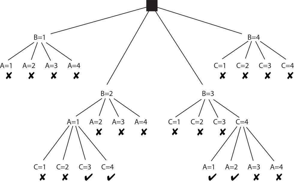
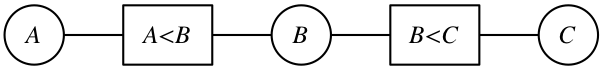
Simple backtracking example
| Variables: | \(A, B, C\) |
| Domains: | \(\mathbf{D}_{A}=\mathbf{D}_{B}=\mathbf{D}_{C}=\{1,2,3,4\}\) |
| Constraints: | \((A<B), (B<C)\) |
Example: Australia map colours
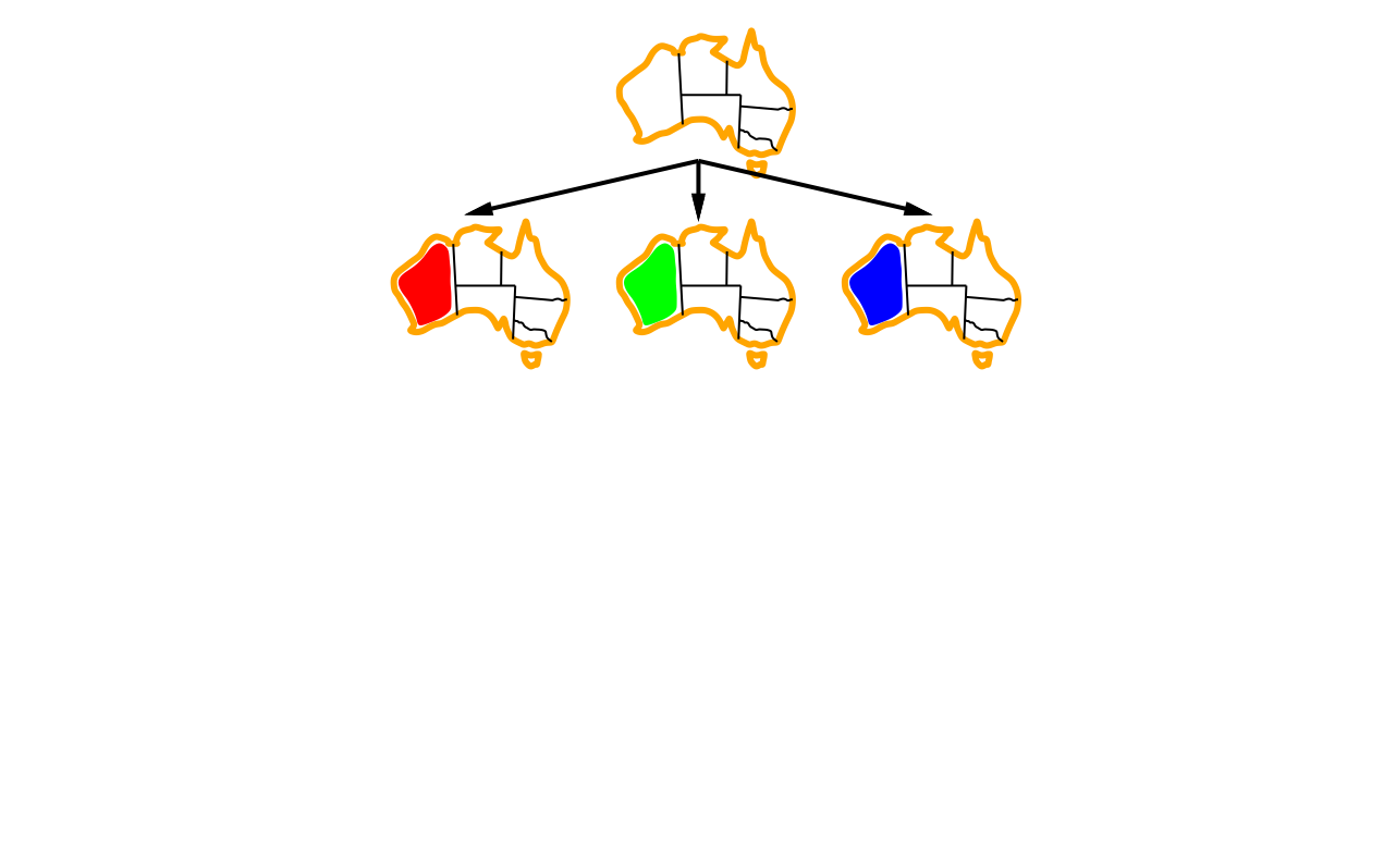
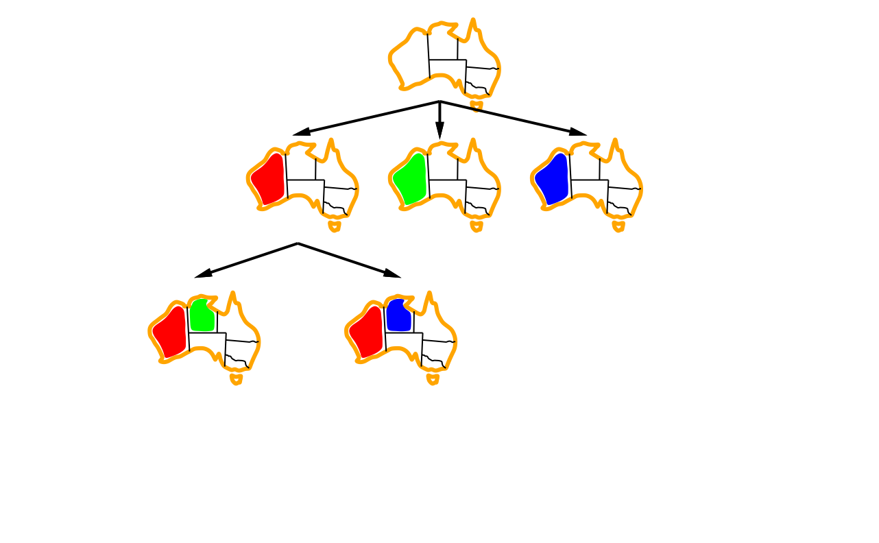
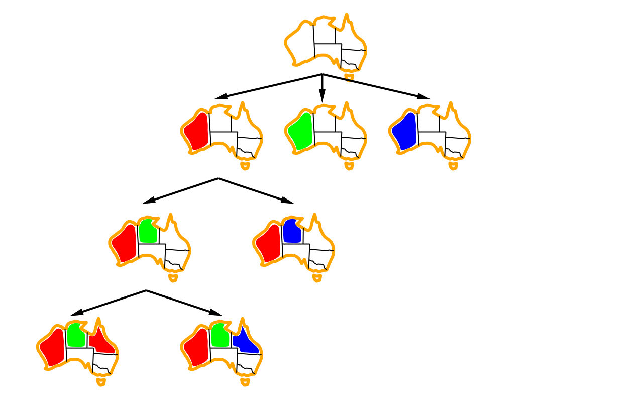
- Assign variable: WA (Western Australia) NT (Northern Territory) Q (Queensland)
Algorithm for backtracking search
- function BacktrackingSearch(csp):
- return Backtrack(csp, { })
- function Backtrack(csp, assignment):
- if assignment is complete then return assignment
- var := SelectUnassignedVariable(csp, assignment)
- for each value in OrderDomainValues(csp, var, assignment):
- if value is consistent with assignment:
- inferences := Inference(csp, var, value)
- if inferences ≠ failure:
- result := Backtrack(csp, assignment \(\cup\) {var=value} \(\cup\) inferences)
- if result ≠ failure then return result
- if value is consistent with assignment:
- return failure
Heuristics: Improving backtracking efficiency
-
The general-purpose algorithm gives rise to several questions:
- Which variable should be assigned next?
- SelectUnassignedVariable(csp, assignment)
- In what order should its values be tried?
- OrderDomainValues(csp, var, assignment)
- What inferences should be performed at each step?
- Inference(csp, var, value)
- Can the search avoid repeating failures?
- Conflict-directed backjumping, constraint learning, no-good sets
(R&N 7.3.3, not covered in this course)
- Conflict-directed backjumping, constraint learning, no-good sets
- Which variable should be assigned next?
Selecting unassigned variables
-
Heuristics for selecting the next unassigned variable:
-
Minimum remaining values (MRV):
\(\Longrightarrow\) choose the variable with the fewest legal values

-
Degree heuristic (if there are several MRV variables):
\(\Longrightarrow\) choose the variable with most constraints on remaining variables

-
Ordering domain values
-
Heuristics for ordering the values of a selected variable:
- Least constraining value:
\(\Longrightarrow\) prefer the value that rules out the fewest choices for the neighboring variables in the constraint graph

- Least constraining value:
Inference: Forward checking
- Forward checking is a simple form of inference:
- Keep track of remaining legal values for unassigned variables
— terminate when any variable has no legal values left - When a new variable is assigned, recalculate the legal values for its neighbors
- Keep track of remaining legal values for unassigned variables
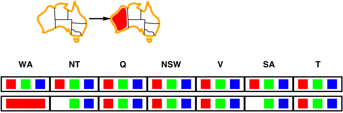
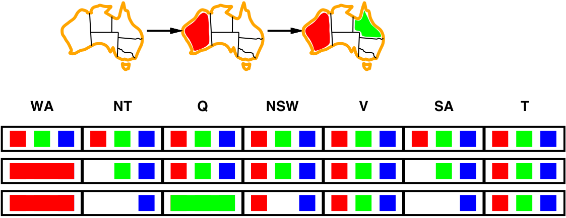
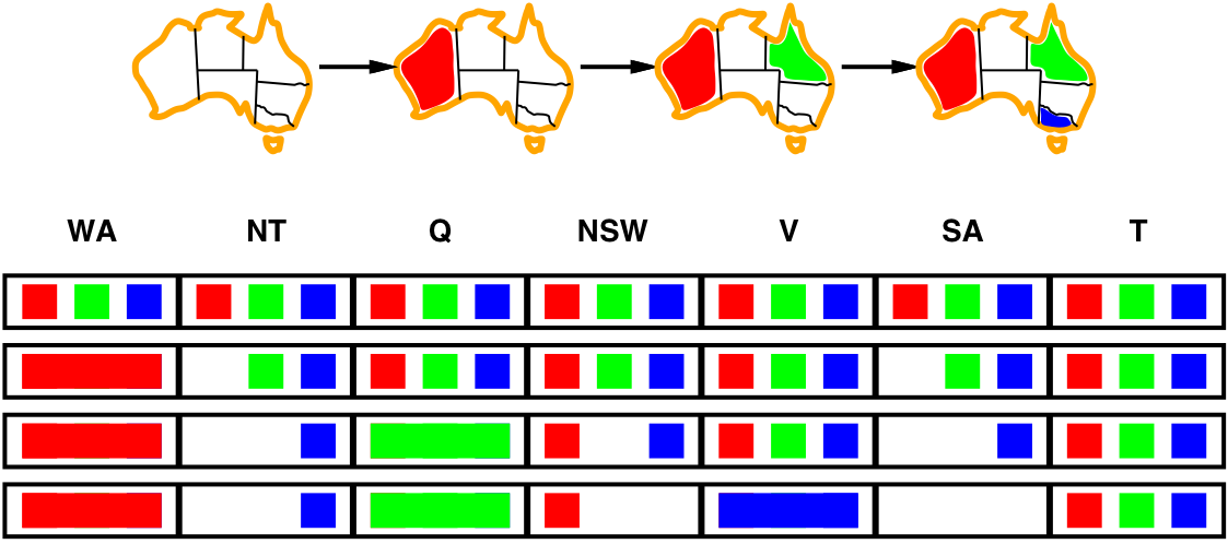
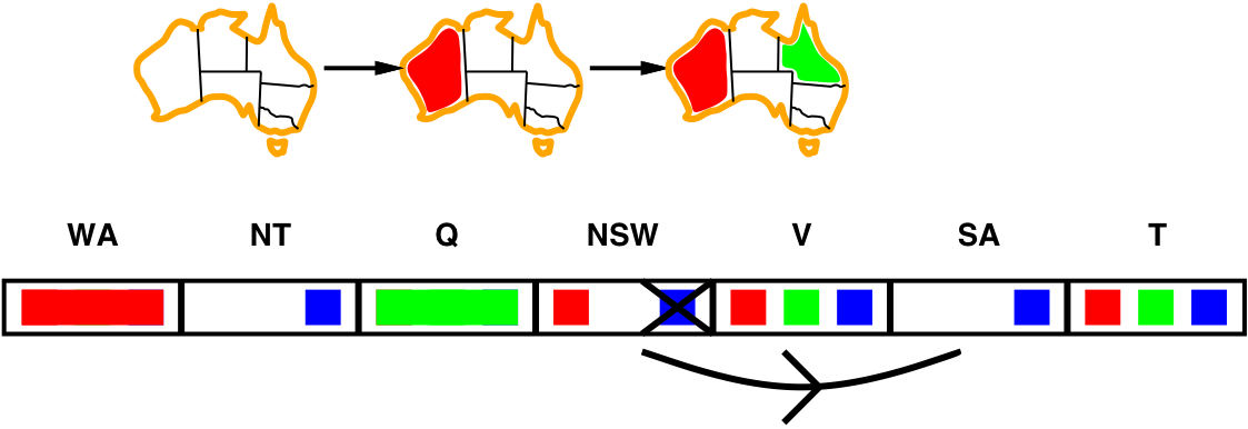
- Colour WA red \(\Longrightarrow\) NT and SA cannot be red
- Colour Q green \(\Longrightarrow\) NT, NSW and SA cannot be green
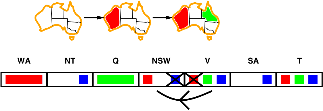
- Colour V blue \(\Longrightarrow\) NSW and SA cannot be blue
\(\Longrightarrow\) SA has no legal values left
Inference: Constraint propagation
-
Forward checking propagates information from assigned to
unassigned variables, but doesn’t detect all failures early:
NT and SA cannot both be blue, but forward checking doesn’t notice that!- Forward checking enforces local constraints
- Constraint propagation enforces local constraints,
repeatedly until reaching a fixed point
Constraint propagation (R&N 7.2–7.2.2)
Arc consistency
Maintaining arc consistency
Constraint propagation: Arc consistency
-
The simplest form of propagation is to make the graph arc consistent:
-
\(X\rightarrow Y\) is arc consistent iff:
for every value \(x\) of \(X\), there is some allowed value \(y\) in \(Y\)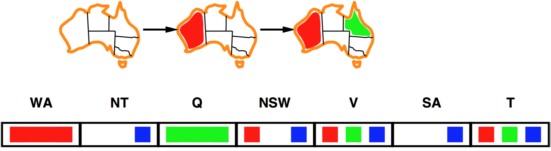

- for every \(x\) in SA, there is an allowed \(y\) in NSW
\(\Longrightarrow\) the arc SA \(\rightarrow\) NSW is consistent - if NSW is blue, there is no allowed color \(y\) in SA
\(\Longrightarrow\) remove blue from NSW - if V is red, there is no allowed color \(y\) in NSW
\(\Longrightarrow\) remove red from V - If \(X\) loses a value, neighbors of \(X\) need to be rechecked
- i.e., the arc SA \(\rightarrow\) NSW must be rechecked
- Arc consistency detects failure earlier than forward checking
-
Consistency
-
Different variants of constistency:
-
A variable is node-consistent if all values in its domain satisfy
its own unary constraints -
a variable is arc-consistent if every value in its domain satisfies
the variable’s binary constraints -
Generalised arc-consistency is the same, but for \(n\)-ary constraints
-
Path consistency is arc-consistency, but for 3 variables at the same time
-
\(k\)-consistency is arc-consistency, but for \(k\) variables
-
…and there are consistency checks for several global constraints,
such as \(\mathit{Alldiff}\) or \(\mathit{Atmost}\)
-
-
A graph is \(X\)-consistent if every variable is \(X\)-consistent with every other variable.
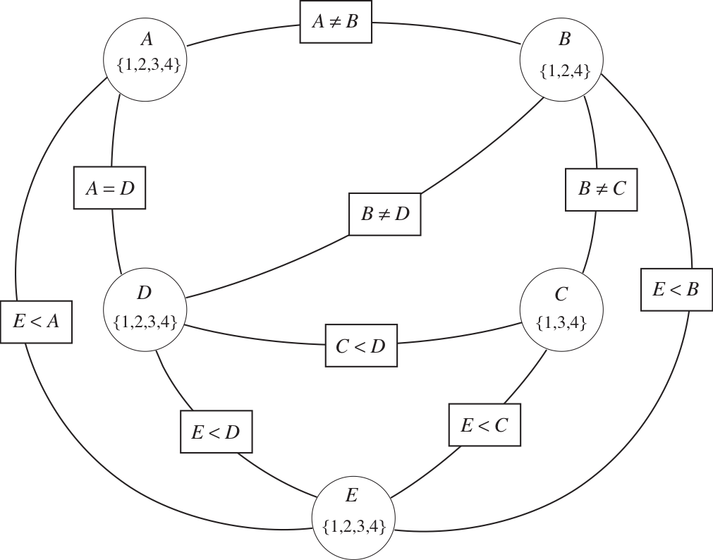
Scheduling example (again)
| Variables: | \(A, B, C, D, E\) representing starting times of various activities. |
| Domains: | \(\mathbf{D}_{A}=\mathbf{D}_{B}=\mathbf{D}_{C}=\mathbf{D}_{D}=\mathbf{D}_{E} = \{1,2,3,4\}\) |
| Constraints: | \((B\neq3), (C\neq2), (A\neq B), (B\neq C), (C<D), (A=D),\) \((E<A), (E<B), (E<C), (E<D), (B\neq D)\) |
-
Is this example node consistent?
-
\(\mathbf{D}_{B}=\{1,2,3,4\}\) is not node consistent,
since \(B=3\) violates the constraint \(B\neq3\)
\(\Longrightarrow\) reduce the domain \(\mathbf{D}_{B}=\{1,2,4\}\) -
\(\mathbf{D}_{C}=\{1,2,3,4\}\) is not node consistent,
since \(C=2\) violates the constraint \(C\neq2\)
\(\Longrightarrow\) reduce the domain \(\mathbf{D}_{C}=\{1,3,4\}\)
-
Scheduling example as a constraint graph
If we reduce the domains for \(B\) and \(C\), then the constraint graph is node consistent.
Arc consistency
- A variable \(X\) is binary arc-consistent with respect to another variable \(Y\) if:
- For each value \(x\in\mathbf{D}_{X}\), there is some \(y\in\mathbf{D}_{Y}\)
such that the binary constraint \(C_{XY}(x,y)\) is satisfied.
- For each value \(x\in\mathbf{D}_{X}\), there is some \(y\in\mathbf{D}_{Y}\)
- A variable \(X\) is generalised arc-consistent with respect to variables \((Y,Z,\dots)\) if:
- For each value \(x\in\mathbf{D}_{X}\), there is some assignment \(y,z,\dots\in\mathbf{D}_{Y},\mathbf{D}_{Z},\dots\) such that \(C_{XYZ\ldots}(x,y,z,\dots)\) is satisfied.
- What if \(X\) is not arc consistent to \(Y\)?
- All values \(x\in\mathbf{D}_{X}\) for which there is no corresponding \(y\in\mathbf{D}_{Y}\)
can be deleted from \(\mathbf{D}_{X}\) to make \(X\) arc consistent.
- All values \(x\in\mathbf{D}_{X}\) for which there is no corresponding \(y\in\mathbf{D}_{Y}\)
- Note! The arcs in a constraint graph are directed:
- \((X,Y)\) and \((Y,X)\) are considered as two different arcs,
- i.e., \(X\) can be arc consistent to \(Y\), but \(Y\) not arc consistent to \(X\).
Arc consistency algorithm
-
Keep a set of arcs to be considered: pick one arc \((X,Y)\) at the time and make it consistent (i.e., make \(X\) arc consistent to \(Y\)).
- Start with the set of all arcs \(\{(X,Y),(Y,X),(X,Z),(Z,X),\ldots\}\).
-
When an arc has been made arc consistent, does it ever need to be checked again?
- An arc \((Z,X)\) needs to be revisited if the domain of \(X\) is changed.
-
Three possible outcomes when all arcs are made arc consistent:
(Is there a solution?)- One domain is empty \(\Longrightarrow\) no solution
- Each domain has a single value \(\Longrightarrow\) unique solution
- Some domains have more than one value \(\Longrightarrow\) maybe a solution, maybe not
Quiz: Arc consistency
-
The variables and constraints are in the constraint graph:
-
Assume the initial domains are \(\mathbf{D}_{A}=\mathbf{D}_{B}=\mathbf{D}_{C}=\{1,2,3,4\}\)
-
How will the domains look like after making the graph arc consistent?
The arc consistency algorithm AC-3
- function AC-3(inout csp):
- initialise queue to all arcs in csp
- while queue is not empty:
- (X, Y) := RemoveOne(queue)
- if Revise(csp, X, Y):
- if \(\mathbf{D}_X=\emptyset\) then return false
- for each Z in X.neighbors–{Y}:
- add (Z, X) to queue
- return true
- function Revise(inout csp, X, Y):
- revised := false
- for each x in \(\mathbf{D}_X\):
- if there is no value y in \(\mathbf{D}_Y\) satisfying the csp constraint \(C_{XY}(x,y)\):
- delete x from \(\mathbf{D}_X\)
- revised := true
- if there is no value y in \(\mathbf{D}_Y\) satisfying the csp constraint \(C_{XY}(x,y)\):
- return revised
- Note: This algorithm destructively updates the domains of the CSP!
You might need to copy the CSP before calling AC-3.
Maintaining arc-consistency (MAC)
-
What if some domains have more than one element after AC?
-
We can always resort to backtracking search:
- Select a variable and a value using some heuristics
(e.g., minimum-remaining-values, degree-heuristic, least-constraining-value) - Make the graph arc-consistent again
- Backtrack and try new values/variables, if AC fails
- Select a new variable/value, perform arc-consistency, etc.
- Select a variable and a value using some heuristics
-
Do we need to restart AC from scratch?
- no, only some arcs risk becoming inconsistent after a new assignment
- restart AC with the queue \(\{(Y_i,X) | X\rightarrow Y_i\}\),
i.e., only the arcs \((Y_i,X)\) where \(Y_i\) are the neighbors of \(X\) - this algorithm is called Maintaining Arc Consistency (MAC)
Domain splitting (not in R&N)
-
What if some domains are very big?
-
Instead of assigning every possible value to a variable, we can split its domain
-
Split one of the domains, then recursively solve each half, i.e.:
- perform AC on the resulting graph, then split a domain,
perform AC, split a domain, perform AC, split, etc.
- perform AC on the resulting graph, then split a domain,
-
It is often good to split a domain in half, i.e.:
- if \(\mathbf{D}_{X}=\{1,\dots,1000\}\), split into \(\{1,\dots500\}\) and \(\{501,\dots,1000\}\)
-