Chapters 4–5: Non-classical and adversarial search
DIT411/TIN175, Artificial Intelligence
Peter Ljunglöf
2 February, 2018
Table of contents
- Repetition
- Non-classical search
- Adversarial search
- Types of games (R&N 5.1)
- Minimax search (R&N 5.2–5.3)
- Minimax search for zero-sum games
- Minimax search: tic-tac-toe
- Minimax example
- Can Minimax be wrong?
- 3-player minimax
- \(\alpha{-}\beta\,\) pruning
- \(\alpha{-}\beta\,\) pruning, general idea
- Minimax example, with \(\alpha{-}\beta\) pruning
- The \(\alpha{-}\beta\) algorithm
- How efficient is \(\alpha{-}\beta\) pruning?
- Minimax and real games
- Imperfect decisions (R&N 5.4–5.4.2)
- Stochastic games (R&N 5.5)
Repetition
Uninformed search (R&N 3.4)
- Search problems, graphs, states, arcs, goal test, generic search algorithm, tree search, graph search, depth-first search, breadth-first search, uniform cost search, iterative deepending, bidirectional search, …
Heuristic search (R&N 3.5–3.6)
- Greedy best-first search, A* search, heuristics, admissibility, consistency, dominating heuristics, …
Local search (R&N 4.1)
- Hill climbing / gradient descent, random moves, random restarts, beam search, simulated annealing, …
Non-classical search
Nondeterministic search (R&N 4.3)
Partial observations (R&N 4.4)
Nondeterministic search (R&N 4.3)
-
- Contingency plan / strategy
- And-or search trees (not in the written exam)
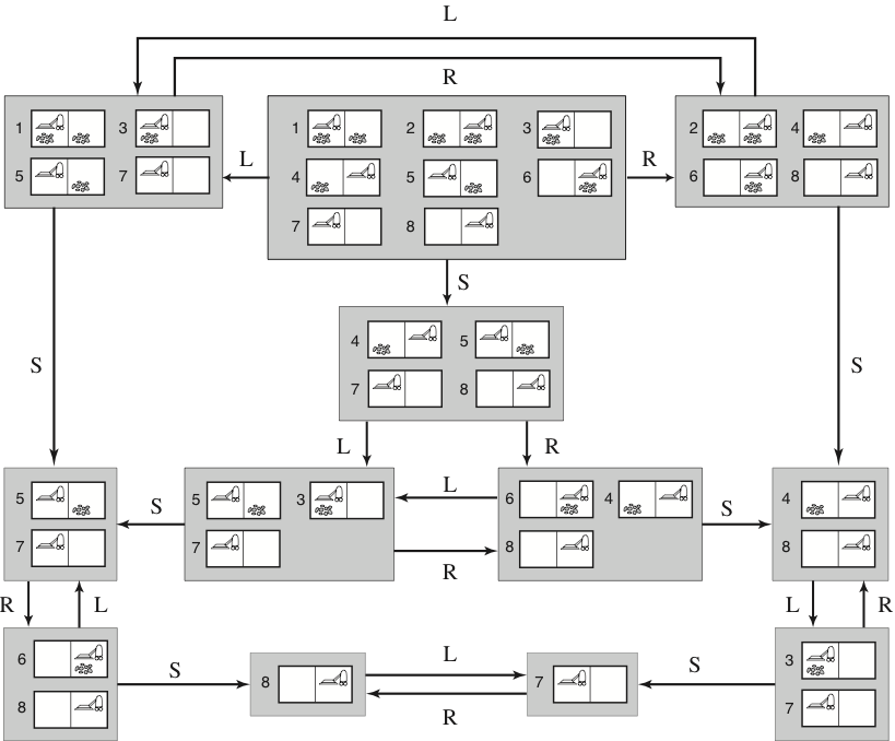
An erratic vacuum cleaner
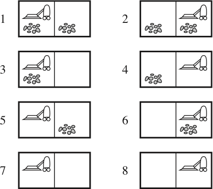
-
The eight possible states of the vacuum world; states 7 and 8 are goal states.
-
There are three actions: Left, Right, Suck.
Assume that the Suck action works as follows:- if the square is dirty, it is cleaned but sometimes also the adjacent square is
- if the square is clean, the vacuum cleaner sometimes deposists dirt
Nondeterministic outcomes, contingency plans
- Assume that the Suck action is nondeterministic:
- if the square is dirty, it is cleaned but sometimes also the adjacent square is
- if the square is clean, the vacuum cleaner sometimes deposists dirt
- Now we need a more general result function:
- instead of returning a single state, it returns a set of possible outcome states
- e.g., \(\textsf{Results}(\textsf{Suck}, 1) = \{5, 7\}\) and \(\textsf{Results}(\textsf{Suck}, 5) = \{1, 5\}\)
- We also need to generalise the notion of a solution:
- instead of a single sequence (path) from the start to the goal,
we need a strategy (or a contingency plan) - i.e., we need if-then-else constructs
- this is a possible solution from state 1:
- [Suck,
ifState=5then[Right, Suck]else[]]
- [Suck,
- instead of a single sequence (path) from the start to the goal,
How to find contingency plans
(will not be in the written examination)
- We need a new kind of nodes in the search tree:
- and nodes:
these are used whenever an action is nondeterministic - normal nodes are called or nodes:
they are used when we have several possible actions in a state
- and nodes:
- A solution for an and-or search problem is a subtree that:
- has a goal node at every leaf
- specifies exactly one action at each of its or node
- includes every branch at each of its and node
A solution to the erratic vacuum cleaner
(will not be in the written examination)
The solution subtree is shown in bold, and corresponds to the plan:
[Suck, if State=5 then [Right, Suck] else []]
An algorithm for finding a contingency plan
(will not be in the written examination)
This algorithm does a depth-first search in the and-or tree,
so it is not guaranteed to find the best or shortest plan:
- function AndOrGraphSearch(problem):
- return OrSearch(problem.InitialState, problem, [])
- function OrSearch(state, problem, path):
- if problem.GoalTest(state) then return []
- if state is on path then return failure
- for each action in problem.Actions(state):
- plan := AndSearch(problem.Results(state, action), problem, [state] ++ path)
- if plan ≠ failure then return [action] ++ plan
- return failure
- function AndSearch(states, problem, path):
- for each \(s_i\) in states:
- \(plan_i\) := OrSearch(\(s_i\), problem, path)
- if \(plan_i\) = failure then return failure
- return [
if\(s_1\)then\(plan_1\)else if\(s_2\)then\(plan_2\)else…if\(s_n\)then\(plan_n\)]
- for each \(s_i\) in states:
While loops in contingency plans
(will not be in the written examination)
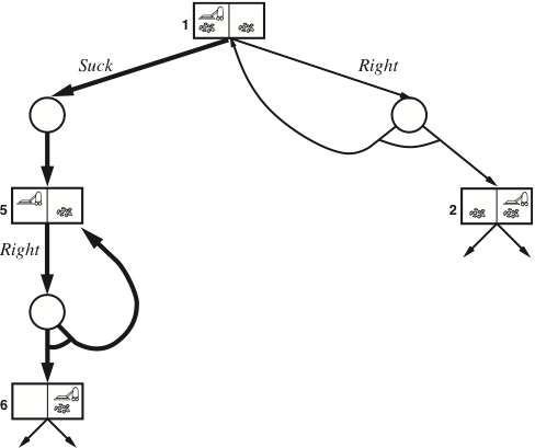
- If the search graph contains cycles, if-then-else is not enough in a contingency plan:
- we need while loops instead
- In the slippery vacuum world above, the cleaner don’t always move when told:
- the solution above translates to [Suck,
whileState=5doRight, Suck]
- the solution above translates to [Suck,
Partial observations (R&N 4.4)
-
- Belief states: goal test, transitions, …
- Sensor-less (conformant) problems
- Partially observable problems
Observability vs determinism
- A problem is nondeterministic if there are several possible outcomes of an action
- deterministic — nondeterministic (chance)
- It is partially observable if the agent cannot tell exactly which state it is in
- fully observable (perfect info.) — partially observable (imperfect info.)
- A problem can be either nondeterministic, or partially observable, or both:

Belief states
- Instead of searching in a graph of states, we use belief states
- A belief state is a set of states
- In a sensor-less (or conformant) problem, the agent has no information at all
- The initial belief state is the set of all problem states
- e.g., for the vacuum world the initial state is {1,2,3,4,5,6,7,8}
- The initial belief state is the set of all problem states
- The goal test has to check that all members in the belief state is a goal
- e.g., for the vacuum world, the following are goal states: {7}, {8}, and {7,8}
- The result of performing an action is the union of all possible results
- i.e., \(\textsf{Predict}(b,a) = \{\textsf{Result}(s,a)\) for each \(s\in b\}\)
- if the problem is also nondeterministic:
- \(\textsf{Predict}(b,a) = \bigcup\{\textsf{Results}(s,a)\) for each \(s\in b\}\)
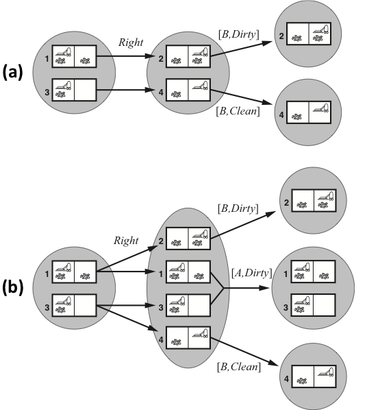
Predicting belief states in the vacuum world
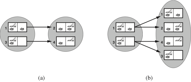
-
(a) Predicting the next belief state for the sensorless vacuum world
with a deterministic action, Right. -
(b) Prediction for the same belief state and action in the nondeterministic
slippery version of the sensorless vacuum world.
The deterministic sensorless vacuum world
Partial observations: state transitions
- With partial observations, we can think of belief state transitions in three stages:
- Prediction, the same as for sensorless problems:
- \(b’ = \textsf{Predict}(b,a) = \{\textsf{Result}(s,a)\) for each \(s\in b\}\)
- Observation prediction, determines the percepts that can be observed:
- \(\textsf{PossiblePercepts}(b’) = \{\textsf{Percept}(s)\) for each \(s\in b’\}\)
- Update, filters the predicted states according to the percepts:
- \(\textsf{Update}(b’,o) = \{s\) for each \(s\in b’\) such that \(o = \textsf{Percept}(s)\}\)
- Prediction, the same as for sensorless problems:
- Belief state transitions:
- \(\textsf{Results}(b,a) = \{\textsf{Update}(b’,o)\) for each \(o\in\textsf{PossiblePercepts}(b’)\}\)
where \(b’ = \textsf{Predict}(b,a)\)
- \(\textsf{Results}(b,a) = \{\textsf{Update}(b’,o)\) for each \(o\in\textsf{PossiblePercepts}(b’)\}\)
Transitions in partially observable vacuum worlds
- The percepts return the current position and the dirtyness of that square.
- The deterministic world:
Right always succeeds. - The slippery world:
Right sometimes fails.
Example: Robot Localisation
The percepts return whether there is a wall in each of the directions.
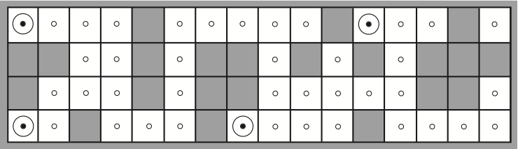
- Possible initial positions of the robot, after E1 = North, South, West.
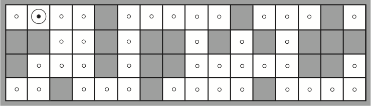
- After moving right and observing E2 = North, South,
there’s only one possible position left.
Adversarial search
Types of games (R&N 5.1)
Minimax search (R&N 5.2–5.3)
Imperfect decisions (R&N 5.4–5.4.2)
Stochastic games (R&N 5.5)
Types of games (R&N 5.1)
-
- cooperative, competetive, zero-sum games
- game trees, ply/plies, utility functions
Multiple agents
-
Let’s consider problems with multiple agents, where:
-
the agents select actions autonomously
- each agent has its own information state
- they can have different information (even conflicting)
-
the outcome depends on the actions of all agents
- each agent has its own utility function (that depends on the total outcome)
-
Types of agents
-
There are two extremes of multiagent systems:
- Cooperative: The agents share the same utility function
- Example: Automatic trucks in a warehouse
- Competetive: When one agent wins all other agents lose
- A common special case is when \(\sum_{a}u_{a}(o)=0\) for any outcome \(o\).
This is called a zero-sum game. - Example: Most board games
- A common special case is when \(\sum_{a}u_{a}(o)=0\) for any outcome \(o\).
- Cooperative: The agents share the same utility function
-
Many multiagent systems are between these two extremes.
- Example: Long-distance bike races are usually both cooperative
(bikers form clusters where they take turns in leading a group),
and competetive (only one of them can win in the end).
- Example: Long-distance bike races are usually both cooperative
Games as search problems
-
The main difference to chapters 3–4:
now we have more than one agent that have different goals.-
All possible game sequences are represented in a game tree.
-
The nodes are states of the game, e.g. board positions in chess.
-
Initial state (root) and terminal nodes (leaves).
-
States are connected if there is a legal move/ply.
(a ply is a move by one player, i.e., one layer in the game tree) -
Utility function (payoff function). Terminal nodes have utility values
\({+}x\) (player 1 wins), \({-}x\) (player 2 wins) and \(0\) (draw).
-
Types of games (again)
Perfect information games: Zero-sum games
-
Perfect information games are solvable in a manner similar to
fully observable single-agent systems, e.g., using forward search. -
If two agents compete, so that a positive reward for one is a negative reward
for the other agent, we have a two-agent zero-sum game. -
The value of a game zero-sum game can be characterised by a single number that one agent is trying to maximise and the other agent is trying to minimise.
-
This leads to a minimax strategy:
- A node is either a MAX node (if it is controlled by the maximising agent),
- or is a MIN node (if it is controlled by the minimising agent).
Minimax search (R&N 5.2–5.3)
-
- Minimax algorithm
- α-β pruning
Minimax search for zero-sum games
- Given two players called MAX and MIN:
- MAX wants to maximise the utility value,
- MIN wants to minimise the same value.
- \(\Rightarrow\) MAX should choose the alternative that maximises, assuming MIN minimises.
- Minimax gives perfect play for deterministic, perfect-information games:
- function Minimax(state):
- if TerminalTest(state) then return Utility(state)
- A := Actions(state)
- if state is a MAX node then return \(\max_{a\in A}\) Minimax(Result(state, a))
- if state is a MIN node then return \(\min_{a\in A}\) Minimax(Result(state, a))
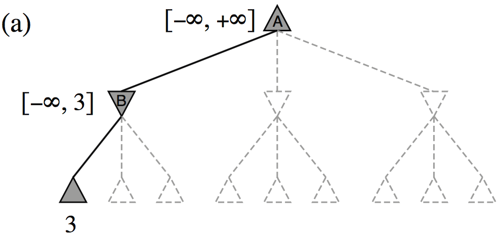
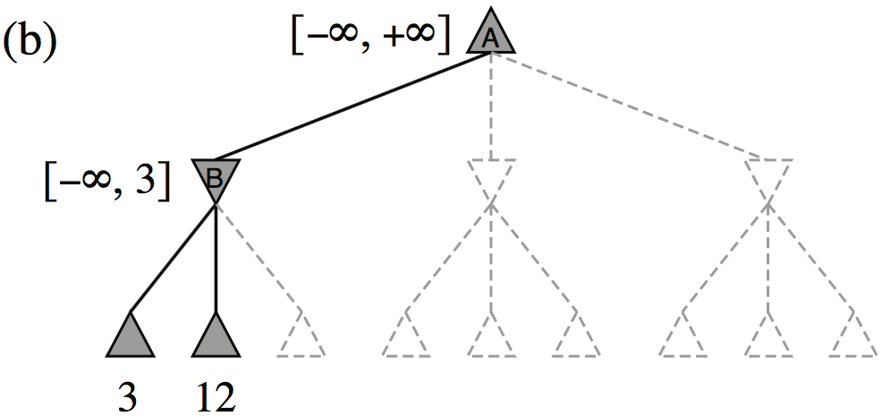
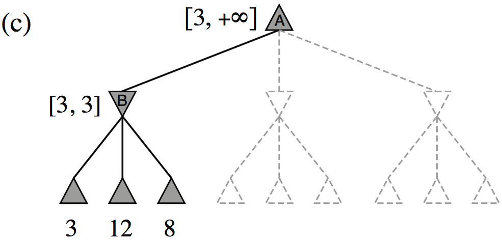
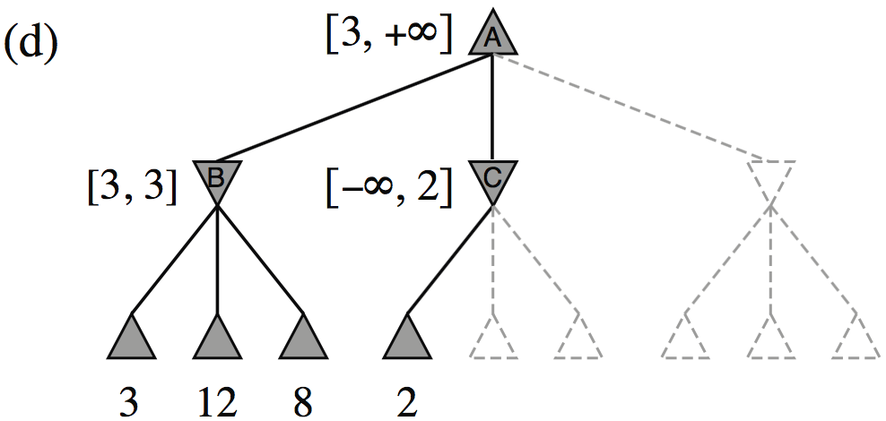
Minimax search: tic-tac-toe

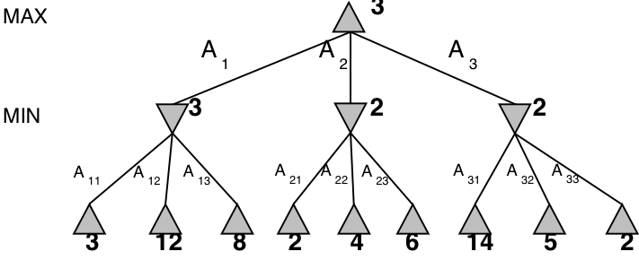
Minimax example
The Minimax algorithm gives perfect play for deterministic, perfect-information games.
Can Minimax be wrong?
- Minimax gives perfect play, but is that always the best strategy?
- Perfect play assumes that the opponent is also a perfect player!
3-player minimax
(will not be in the written examination)
Minimax can also be used on multiplayer games
\(\alpha{-}\beta\,\) pruning
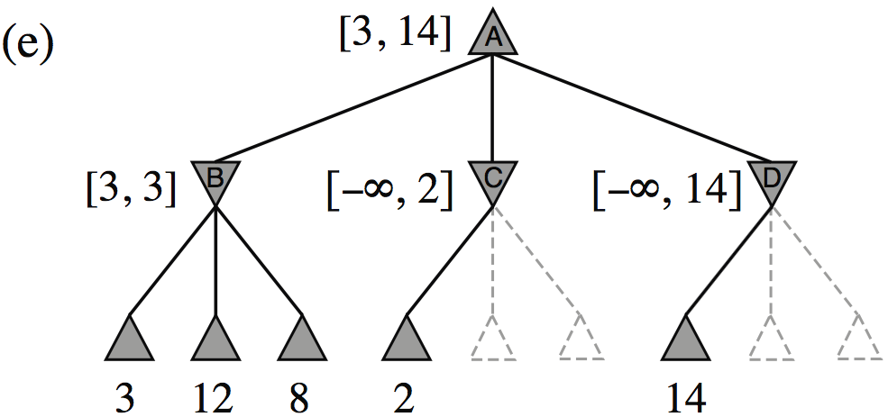
| Minimax(root) | = | \( \max(\min(3,12,8), \min(2,x,y), \min(14,5,2)) \) |
| = | \( \max(3, \min(2,x,y), 2) \) | |
| = | \( \max(3, z, 2) \) where \(z = \min(2,x,y) \leq 2\) | |
| = | \( 3 \) |
- I.e., we don’t need to know the values of \(x\) and \(y\)!
\(\alpha{-}\beta\,\) pruning, general idea
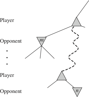
- The general idea of α-β pruning is this:
- • if \(m\) is better than \(n\) for Player,
- we don’t want to pursue \(n\)
- • so, once we know enough about \(n\)
- we can prune it
- • sometimes it’s enough to examine
- just one of \(n\)’s descendants
- α-β pruning keeps track of the possible range
of values for every node it visits;
the parent range is updated when the child has been visited.
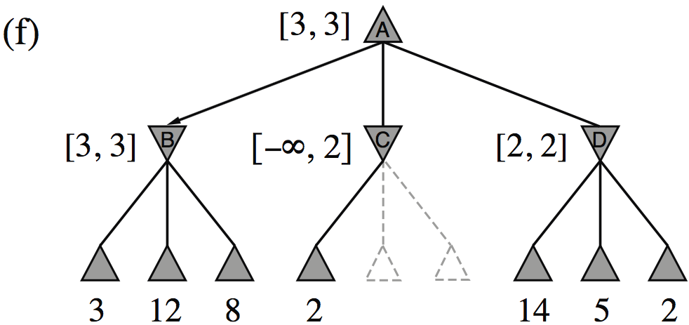
Minimax example, with \(\alpha{-}\beta\) pruning
The \(\alpha{-}\beta\) algorithm
- function AlphaBetaSearch(state):
- v := MaxValue(state, \(-\infty\), \(+\infty\)))
- return the action in Actions(state) that has value v
- function MaxValue(state, α, β):
- if TerminalTest(state) then return Utility(state)
- v := \(-\infty\)
- for each action in Actions(state):
- v := max(v, MinValue(Result(state, action), α, β))
- if v ≥ β then return v
- α := max(α, v)
- return v
- function MinValue(state, α, β):
- same as MaxValue but reverse the roles of α/β and min/max and \(-\infty/{+}\infty\)
How efficient is \(\alpha{-}\beta\) pruning?
-
The amount of pruning provided by the α-β algorithm depends on the ordering of the children of each node.
-
It works best if a highest-valued child of a MAX node is selected first and
if a lowest-valued child of a MIN node is selected first. -
In real games, much of the effort is made to optimise the search order.
-
With a “perfect ordering”, the time complexity becomes \(O(b^{m/2})\)
- this doubles the solvable search depth
- however, \(35^{80/2}\) (for chess) or \(250^{160/2}\) (for go) is still quite large…
-
Minimax and real games
-
Most real games are too big to carry out minimax search, even with α-β pruning.
-
For these games, instead of stopping at leaf nodes,
we have to use a cutoff test to decide when to stop. -
The value returned at the node where the algorithm stops
is an estimate of the value for this node. -
The function used to estimate the value is an evaluation function.
-
Much work goes into finding good evaluation functions.
-
There is a trade-off between the amount of computation required
to compute the evaluation function and the size of the search space
that can be explored in any given time.
-
Imperfect decisions (R&N 5.4–5.4.2)
-
- H-minimax algorithm
- evaluation function, cutoff test
- features, weighted linear function
- quiescence search, horizon effect
H-minimax algorithm
- The Heuristic Minimax algorithm is similar to normal Minimax
- it replaces TerminalTest with CutoffTest, and Utility with Eval
- the cutoff test needs to know the current search depth
- function H-Minimax(state, depth):
- if CutoffTest(state, depth) then return Eval(state)
- A := Actions(state)
- if state is a MAX node then return \(\max_{a\in A}\) H-Minimax(Result(state, a), depth+1)
- if state is a MIN node then return \(\min_{a\in A}\) H-Minimax(Result(state, a), depth+1)
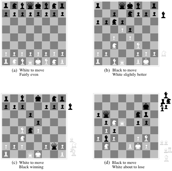
Chess positions: how to evaluate
Weighted linear evaluation functions
-
A very common evaluation function is to use a weighted sum of features: \[ Eval(s) = w_1 f_1(s) + w_2 f_2(s) + \cdots + w_n f_n(s) = \sum_{i=1}^{n} w_i f_i(s) \]
- This relies on a strong assumption: all features are independent of each other
- which is usually not true, so the best programs for chess
(and other games) also use nonlinear feature combinations
- which is usually not true, so the best programs for chess
- The weights can be calculated using machine learning algorithms,
but a human still has to come up with the features.- using recent advances in deep machine learning,
the computer can learn the features too
- using recent advances in deep machine learning,
Evaluation functions
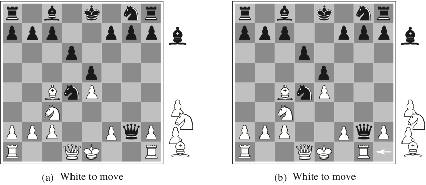
A naive weighted sum of features will not see the difference between these two states.
Problems with cutoff tests
- Too simplistic cutoff tests and evaluation functions can be problematic:
- e.g., if the cutoff is only based on the current depth
- then it might cut off the search in unfortunate positions
(such as (b) on the previous slide)
- We want more sophisticated cutoff tests:
- only cut off search in quiescent positions
- i.e., in positions that are “stable”, unlikely to exhibit wild swings in value
- non-quiescent positions should be expanded further
- Another problem is the horizon effect:
- if a bad position is unavoidable (e.g., loss of a piece), but the system can
delay it from happening, it might push the bad position “over the horizon” - in the end, the resulting delayed position might be even worse
- if a bad position is unavoidable (e.g., loss of a piece), but the system can
Deterministic games in practice
- Chess:
- IBM DeepBlue beats world champion Garry Kasparov, 1997.
- Google AlphaZero beats best chess program Stockfish, December 2017.
- Checkers/Othello/Reversi:
- Logistello beats the world champion in Othello/Reversi, 1997.
- Chinook plays checkers perfectly, 2007. It uses an endgame database
defining perfect play for all 8-piece positions on the board,
(a total of 443,748,401,247 positions).
- Go:
- First Go programs to reach low dan-levels, 2009.
- Google AlphaGo beats the world’s best Go player, Ke Jie, May 2017.
- Google AlphaZero beats AlphaGo, December 2017.
- AlphaZero learns board game strategies by playing itself, it does not use a database of previous matches, opening books or endgame tables.
Stochastic games (R&N 5.5)
Note: this section will be presented Tuesday 6th February!