Chapters 5, 7: Search part IV, and CSP, part II
DIT411/TIN175, Artificial Intelligence
Peter Ljunglöf
6 February, 2018
Table of contents
Repetition of search
Classical search (R&N 3.1–3.6)
- Generic search algorithm, tree search, graph search, depth-first search,
breadth-first search, uniform cost search, iterative deepending,
bidirectional search, greedy best-first search, A* search,
heuristics, admissibility, consistency, dominating heuristics, …
Non-classical search (R&N 4.1, 4.3–4.4)
- Hill climbing, random moves, random restarts, beam search,
nondeterministic actions, contingency plan, and-or search trees,
partial observations, belief states, sensor-less problems, …
Adversarial search (R&N 5.1–5.4)
- Cooperative, competetive, zero-sum games, game trees, minimax,
α-β pruning, H-minimax, evaluation function, cutoff test,
features, weighted linear function, quiescence search, horizon effect, …
More games
Stochastic games (R&N 5.5)
Repetition: Minimax search for zero-sum games
- Given two players called MAX and MIN:
- MAX wants to maximise the utility value,
- MIN wants to minimise the same value.
- \(\Rightarrow\) MAX should choose the alternative that maximises, assuming MIN minimises.
- function Minimax(state):
- if TerminalTest(state) then return Utility(state)
- A := Actions(state)
- if state is a MAX node then return \(\max_{a\in A}\) Minimax(Result(state, a))
- if state is a MIN node then return \(\min_{a\in A}\) Minimax(Result(state, a))
Repetition: H-minimax algorithm
- The Heuristic Minimax algorithm is similar to normal Minimax
- it replaces TerminalTest with CutoffTest, and Utility with Eval
- the cutoff test needs to know the current search depth
- function H-Minimax(state, depth):
- if CutoffTest(state, depth) then return Eval(state)
- A := Actions(state)
- if state is a MAX node then return \(\max_{a\in A}\) H-Minimax(Result(state, a), depth+1)
- if state is a MIN node then return \(\min_{a\in A}\) H-Minimax(Result(state, a), depth+1)
Repetition: The \(\alpha{-}\beta\) algorithm
- function AlphaBetaSearch(state):
- v := MaxValue(state, \(-\infty\), \(+\infty\)))
- return the action in Actions(state) that has value v
- function MaxValue(state, α, β):
- if TerminalTest(state) then return Utility(state)
- v := \(-\infty\)
- for each action in Actions(state):
- v := max(v, MinValue(Result(state, action), α, β))
- if v ≥ β then return v
- α := max(α, v)
- return v
- function MinValue(state, α, β):
- same as MaxValue but reverse the roles of α/β and min/max and \(-\infty/{+}\infty\)
Stochastic games (R&N 5.5)
-
- chance nodes
- expected value
- expecti-minimax algorithm
Games of imperfect information
-
Imperfect information games
-
e.g., card games, where the opponent’s initial cards are unknown
-
typically we can calculate a probability for each possible deal
-
seems just like having one big dice roll at the beginning of the game
-
main idea: compute the minimax value of each action in each deal,
then choose the action with highest expected value over all deals
-
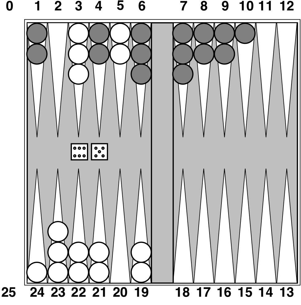
Stochastic game example: Backgammon
Stochastic games in general
- In stochastic games, chance is introduced by dice, card-shuffling, etc.
- We introduce chance nodes to the game tree.
- We can’t calculate a definite minimax value,
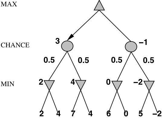
instead we calculate the expected value of a position. - The expected value is the average of all possible outcomes.
- A very simple example with coin-flipping and arbitrary values:
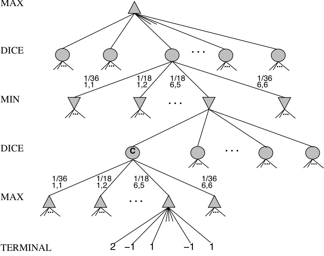
Backgammon game tree
Algorithm for stochastic games
- The ExpectiMinimax algorithm gives perfect play;
- it’s just like Minimax, except we must also handle chance nodes:
- function ExpectiMinimax(state):
- if TerminalTest(state) then return Utility(state)
- A := Actions(state)
- if state is a MAX node then return \(\max_{a\in A}\) ExpectiMinimax(Result(state, a))
- if state is a MAX node then return \(\min_{a\in A}\) ExpectiMinimax(Result(state, a))
- if state is a chance node then return \(\sum_{a\in A}P(a)\)·ExpectiMinimax(Result(state, a))
where \(P(a)\) is the probability that action a occurs.
Stochastic games in practice
- Dice rolls increase the branching factor:
- there are 21 possible rolls with 2 dice
- Backgammon has ≈20 legal moves:
- depth \(4\Rightarrow20\times(21\times20)^{3}\approx1.2\times10^{9}\) nodes
- As depth increases, the probability of reaching a given node shrinks:
- value of lookahead is diminished
- α-β pruning is much less effective
- TD-Gammon (1995) used depth-2 search + very good Eval function:
- the evaluation function was learned by self-play
- world-champion level
Repetition of CSP
Constraint satisfaction problems (R&N 7.1)
- Variables, domains, constraints (unary, binary, n-ary), constraint graph
CSP as a search problem (R&N 7.3–7.3.2)
- Backtracking search, heuristics (minimum remaining values, degree, least constraining value), forward checking, maintaining arc-consistency (MAC)
Constraint propagation (R&N 7.2–7..2.2)
- Consistency (node, arc, path, k, …), global constratints, the AC-3 algorithm
CSP: Constraint satisfaction problems (R&N 7.1)
- CSP is a specific kind of search problem:
- the state is defined by variables \(X_{i}\), each taking values from the domain \(D_{i}\)
- the goal test is a set of constraints:
- each constraint specifies allowed values for a subset of variables
- all constraints must be satisfied
- Differences to general search problems:
- the path to a goal isn’t important, only the solution is.
- there are no predefined starting state
- often these problems are huge, with thousands of variables,
so systematically searching the space is infeasible
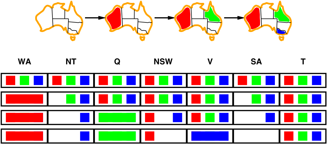
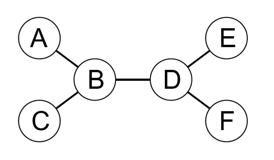
Example: Map colouring (binary CSP)
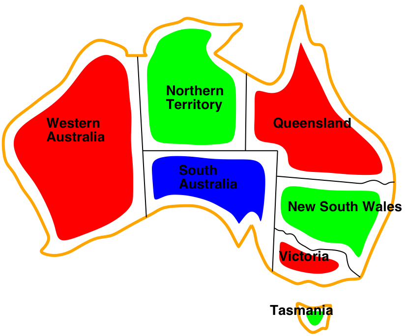
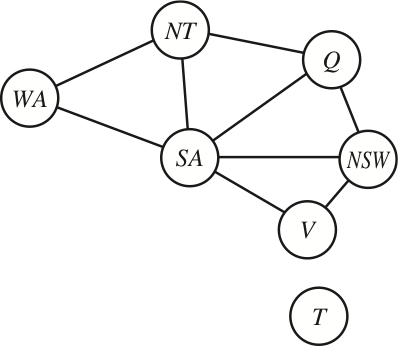
| Variables: | WA, NT, Q, NSW, V, SA, T |
| Domains: | \(D_i\) = {red, green, blue} |
| Constraints: | SA≠WA, SA≠NT, SA≠Q, SA≠NSW, SA≠V, WA≠NT, NT≠Q, Q≠NSW, NSW≠V |
| Constraint graph: | Every variable is a node, every binary constraint is an arc. |
Example: Cryptarithmetic puzzle (higher-order CSP)
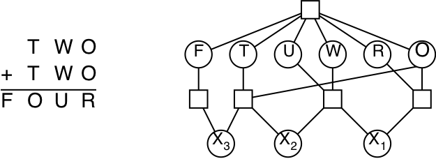
| Variables: | F, T, U, W, R, O, \(X_1, X_2, X_3\) |
| Domains: | \(D_i\) = {0, 1, 2, 3, 4, 5, 6, 7, 8, 9} |
| Constraints: | Alldiff(F,T,U,W,R,O), O+O=R+10·\(X_1\), etc. |
| Constraint graph: | This is not a binary CSP! The graph is a constraint hypergraph. |
CSP as a search problem (R&N 7.3–7.3.2)
-
- backtracking search
- select variable: minimum remaining values, degree heuristic
- order domain values: least constraining value
- inference: forward checking and arc consistency
Algorithm for backtracking search
- At each depth level, decide on one single variable to assign:
- this gives branching factor \(b=d\), so there are \(d^{n}\) leaves
- Depth-first search with single-variable assignments is called backtracking search:
- function BacktrackingSearch(csp):
- return Backtrack(csp, { })
- function Backtrack(csp, assignment):
- if assignment is complete then return assignment
- var := SelectUnassignedVariable(csp, assignment)
- for each value in OrderDomainValues(csp, var, assignment):
- if value is consistent with assignment:
- inferences := Inference(csp, var, value)
- if inferences ≠ failure:
- result := Backtrack(csp, assignment \(\cup\) {var=value} \(\cup\) inferences)
- if result ≠ failure then return result
- if value is consistent with assignment:
- return failure
Improving backtracking efficiency
-
The general-purpose algorithm gives rise to several questions:
- Which variable should be assigned next?
- SelectUnassignedVariable(csp, assignment)
- In what order should its values be tried?
- OrderDomainValues(csp, var, assignment)
- What inferences should be performed at each step?
- Inference(csp, var, value)
- Can the search avoid repeating failures?
- Conflict-directed backjumping, constraint learning, no-good sets
(R&N 7.3.3, not covered in this course)
- Conflict-directed backjumping, constraint learning, no-good sets
- Which variable should be assigned next?
Selecting unassigned variables
-
Heuristics for selecting the next unassigned variable:
-
Minimum remaining values (MRV):
\(\Longrightarrow\) choose the variable with the fewest legal values

-
Degree heuristic (if there are several MRV variables):
\(\Longrightarrow\) choose the variable with most constraints on remaining variables

-
Ordering domain values
-
Heuristics for ordering the values of a selected variable:
- Least constraining value:
\(\Longrightarrow\) prefer the value that rules out the fewest choices
for the neighboring variables in the constraint graph

- Least constraining value:
Constraint propagation (R&N 7.2–7.2.2)
-
- consistency (node, arc, path, k, …)
- global constratints
- the AC-3 algorithm
- maintaining arc consistency
Inference: Forward checking and arc consistency
- Forward checking is a simple form of inference:
- Keep track of remaining legal values for unassigned variables
- When a new variable is assigned, recalculate the legal values for its neighbors
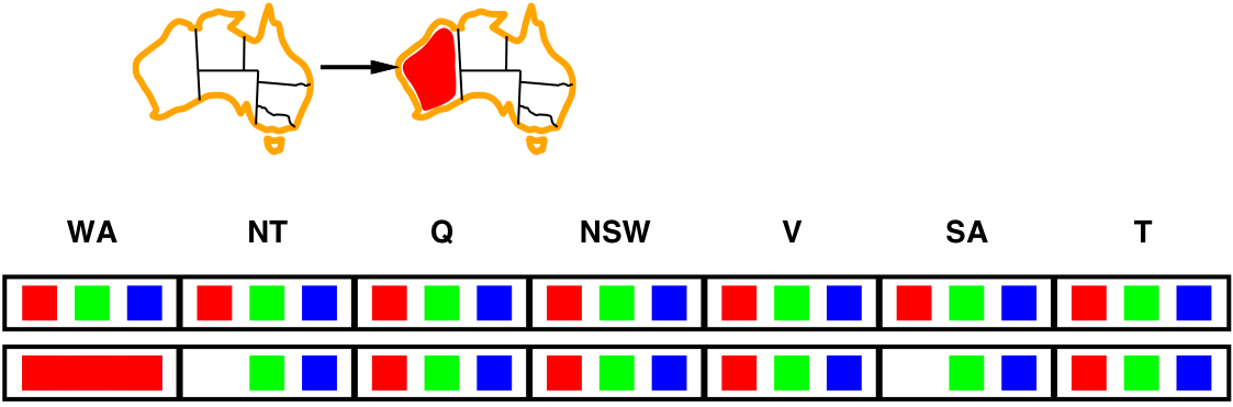
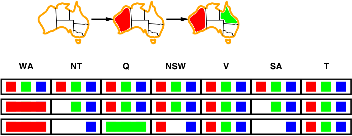
- Arc consistency: \(X\rightarrow Y\) is ac iff for every \(x\) in \(X\), there is some allowed \(y\) in \(Y\)
- since NT and SA cannot both be blue, the problem becomes
arc inconsistent before forward checking notices - arc consistency detects failure earlier than forward checking
- since NT and SA cannot both be blue, the problem becomes
Arc consistency algorithm, AC-3
- Keep a set of arcs to be considered: pick one arc \((X,Y)\) at the time and
make it consistent (i.e., make \(X\) arc consistent to \(Y\)).
- Start with the set of all arcs \(\{(X,Y),(Y,X),(X,Z),(Z,X),\ldots\}\).
- When an arc has been made arc consistent, does it ever need to be checked again?
- An arc \((Z,X)\) needs to be revisited if the domain of \(X\) is revised.
- function AC-3(inout csp):
- initialise queue to all arcs in csp
- while queue is not empty:
- (X, Y) := RemoveOne(queue)
- if Revise(csp, X, Y):
- if \(D_X=\emptyset\) then return failure
- for each Z in X.neighbors–{Y} do add (Z, X) to queue
- function Revise(inout csp, X, Y):
- delete every x from \(D_X\) such that there is no value y in \(D_Y\) satisfying the constraint \(C_{XY}\)
- return true if \(D_X\) was revised
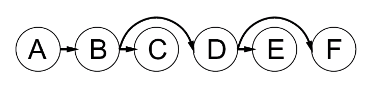
AC-3 example
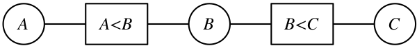
| remove | \(D_A\) | \(D_B\) | \(D_C\) | add | queue |
|---|---|---|---|---|---|
| 1234 | 1234 | 1234 | A<B, B<C, C>B, B>A | ||
| A<B | 123 | 1234 | 1234 | B<C, C>B, B>A | |
| B<C | 123 | 123 | 1234 | A<B | C>B, B>A, A<B |
| C>B | 123 | 123 | 234 | B>A, A<B | |
| B>A | 123 | 23 | 234 | C>B | A<B, C>B |
| A<B | 12 | 23 | 234 | C>B | |
| C>B | 12 | 23 | 34 | \(\emptyset\) | |
Combining backtracking with AC-3
-
What if some domains have more than one element after AC?
-
We can resort to backtracking search:
- Select a variable and a value using some heuristics
(e.g., minimum-remaining-values, degree-heuristic, least-constraining-value) - Make the graph arc-consistent again
- Backtrack and try new values/variables, if AC fails
- Select a new variable/value, perform arc-consistency, etc.
- Select a variable and a value using some heuristics
-
Do we need to restart AC from scratch?
- no, only some arcs risk becoming inconsistent after a new assignment
- restart AC with the queue \(\{(Y_i,X) \;|\; X\rightarrow Y_i\}\),
i.e., only the arcs \((Y_i,X)\) where \(Y_i\) are the neighbors of \(X\) - this algorithm is called Maintaining Arc Consistency (MAC)
Consistency properties
-
There are several kinds of consistency properties and algorithms:
-
Node consistency: single variable, unary constraints (straightforward)
-
Arc consistency: pairs of variables, binary constraints (AC-3 algorithm)
-
Path consistency: triples of variables, binary constraints (PC-2 algorithm)
-
\(k\)-consistency: \(k\) variables, \(k\)-ary constraints (algorithms exponential in \(k\))
-
Consistency for global constraints:
Special-purpose algorithms for different constraints, e.g.:- Alldiff(\(X_1,\ldots,X_m\)) is inconsistent if \(m > |D_1\cup\cdots\cup D_m|\)
- Atmost(\(n,X_1,\ldots,X_m\)) is inconsistent if \(n < \sum_i \min(D_i)\)
-
More about CSP
Local search for CSP (R&N 7.4)
Problem structure (R&N 7.5)
Local search for CSP (R&N 7.4)
- Given an assignment of a value to each variable:
- A conflict is an unsatisfied constraint.
- The goal is an assignment with zero conflicts.
- Local search / Greedy descent algorithm:
- Start with a complete assignment.
- Repeat until a satisfying assignment is found:
- select a variable to change
- select a new value for that variable
Min conflicts algorithm
- Heuristic function to be minimised: the number of conflicts.
- this is the min-conflicts heuristics
- Note: this does not always work!
- it can get stuck in a local minimum
- function MinConflicts(csp, max_steps)
- current := an initial complete assignment for csp
- repeat max_steps times:
- if current is a solution for csp then return current
- var := a randomly chosen conflicted variable from csp
- value := the value v for var that minimises Conflicts(var, v, current, csp)
- current[var] = value
- return failure
Example: \(n\)-queens (revisited)
-
Do you remember this example?
- Put \(n\) queens on an \(n\times n\) board, in separate columns
- Conflicts = unsatisfied constraints = n:o of threatened queens
- Move a queen to reduce the number of conflicts
- repeat until we cannot move any queen anymore
- then we are at a local maximum — hopefully it is global too
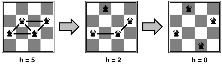
Easy and hard problems
- Two-step solution using min-conflicts for an 8-queens problem:
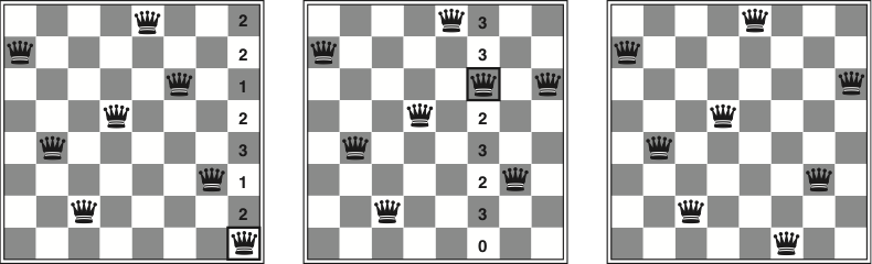
- The runtime of min-conflicts on n-queens is independent of problem size!
- it solves even the million-queens problem ≈50 steps
- Why is n-queens easy for local search?
- because solutions are densely distributed throughout the state space!
Variants of greedy descent
-
To choose a variable to change and a new value for it:
- Find a variable-value pair that minimises the number of conflicts.
- Select a variable that participates in the most conflicts.
Select a value that minimises the number of conflicts. - Select a variable that appears in any conflict.
Select a value that minimises the number of conflicts. - Select a variable at random.
Select a value that minimises the number of conflicts. - Select a variable and value at random;
accept this change if it doesn’t increase the number of conflicts.
-
All local search techniques from section 4.1 can be applied to CSPs, e.g.:
- random walk, random restarts, simulated annealing, beam search, …
Problem structure (R&N 7.5)
(will not be in the written examination)
-
- independent subproblems, connected components
- tree-structured CSP, topological sort
- converting to tree-structured CSP, cycle cutset, tree decomposition
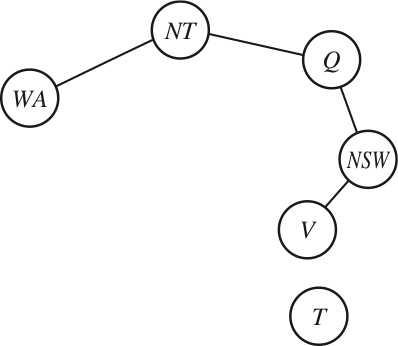
Independent subproblems
-
- Tasmania is an independent subproblem:
- there are efficient algorithms for finding connected components in a graph
-
Suppose that each subproblem has \(c\) variables out of \(n\) total. The cost of the worst-case solution
is \(n/c\cdot d^{c}\), which is linear in \(n\). - E.g., \(n=80, d=2, c=20\):
- \(2^{80}\) = 4 billion years at 10 million nodes/sec
- If we divide it into 4 equal-size subproblems:
- \(4\cdot2^{20}\) =0.4 seconds at 10 million nodes/sec
- Note: this only has a real effect if the subproblems are (roughly) equal size!
Tree-structured CSP
- A constraint graph is a tree when any two variables are connected by only one path.
- then any variable can act as root in the tree
- tree-structured CSP can be solved in linear time, in the number of variables!
- To solve a tree-structured CSP:
- first pick a variable to be the root of the tree
- then find a topological sort of the variables (with the root first)
- finally, make each arc consistent, in reverse topological order
Solving tree-structured CSP
- function TreeCSPSolver(csp)
- n := number of variables in csp
- root := any variable in csp
- \(X_1\ldots X_n\) := TopologicalSort(csp, root)
- for j := n, n–1, …, 2:
- MakeArcConsistent(Parent(\(X_j\)), \(X_j\))
- if it could not be made consistent then return failure
- assignment := an empty assignment
- for i := 1, 2, …, n:
- assignment[\(X_i\)] := any consistent value from \(D_i\)
- return assignment
- What is the runtime?
- to make an arc consistent, we must compare up to \(d^2\) domain value pairs
- there are \(n{-}1\) arcs, so the total runtime is \(O(nd^2)\)
Converting to tree-structured CSP
- Most CSPs are not tree-structured, but sometimes we can reduce them to a tree
- one approach is to assign values to some variables,
so that the remaining variables form a tree
- one approach is to assign values to some variables,
-
If we assign a colour to South Australia, then the remaining variables form a tree
-
A (worse) alternative is to assign values to {NT,Q,V}
- Why is {NT,Q,V} a worse alternative?
- Because then we have to try 3×3×3 different assignments,
and for each of them solve the remaining tree-CSP
Solving almost-tree-structured CSP
- function SolveByReducingToTreeCSP(csp):
- S := a cycle cutset of variables, such that csp–S becomes a tree
- for each assignment for S that satisfies all constraints on S:
- remove any inconsistent values from neighboring variables of S
- solve the remaining tree-CSP (i.e., csp–S)
- if there is a solution then return it together with the assignment for S
- return failure
- The set of variables that we have to assign is called a cycle cutset
- for Australia, {SA} is a cycle cutset and {NT,Q,V} is also a cycle cutset
- finding the smallest cycle cutset is NP-hard,
but there are efficient approximation algorithms