Chapters 3, 4, 5, 7: Repetition
DIT411/TIN175, Artificial Intelligence
Peter Ljunglöf
9 February, 2018
Table of contents
- Search (R&N 3.1–3.6, 4.1, 4.3–4.4)
- Uninformed search
- Directed Graphs
- How do we search in a graph?
- Illustration of searching in a graph
- The generic tree search algorithm
- Using tree search on a graph
- Turning tree search into graph search
- Tree search vs. graph search
- Depth-first and breadth-first search
- Iterative deepening
- Iterative deepening complexity
- Bidirectional search
- Cost-based search
- The frontier is a Priority Queue, ordered by \(f(n)\)
- A* tree search is optimal!
- The generic tree search algorithm
- Turning tree search into graph search
- Graph-search = Multiple-path pruning
- When is A* graph search optimal?
- State-space contours
- Summary of optimality of A*
- Summary of tree search strategies
- Summary of graph search strategies
- Heuristics
- Non-classical search
- Uninformed search
- Adversarial search (R&N 5.1–5.5)
- Constraint satisfaction problems (R&N 4.1, 7.1–7.5)
Search (R&N 3.1–3.6, 4.1, 4.3–4.4)
Uninformed search
Cost-based search
Heuristics
Non-classical search
Directed Graphs
-
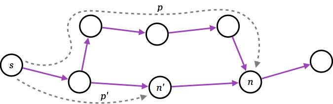
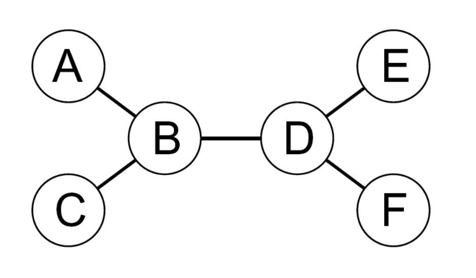
A graph consists of a set \(N\) of nodes and a set \(A\) of ordered pairs of nodes,
called arcs or edges.-
Node \(n_2\) is a neighbor of \(n_1\) if there is an arc from \(n_1\) to \(n_2\).
That is, if \( (n_1, n_2) \in A \). -
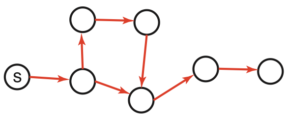
A path is a sequence of nodes \( (n_0, n_1, \ldots, n_k) \) such that \( (n_{i-1}, n_i) \in A \).
-
The length of path \( (n_0, n_1, \ldots, n_k) \) is \(k\).
-
A solution is a path from a start node to a goal node,
given a set of start nodes and goal nodes. -
(Russel & Norvig sometimes call the graph nodes states).
-
How do we search in a graph?
-
A generic search algorithm:
-
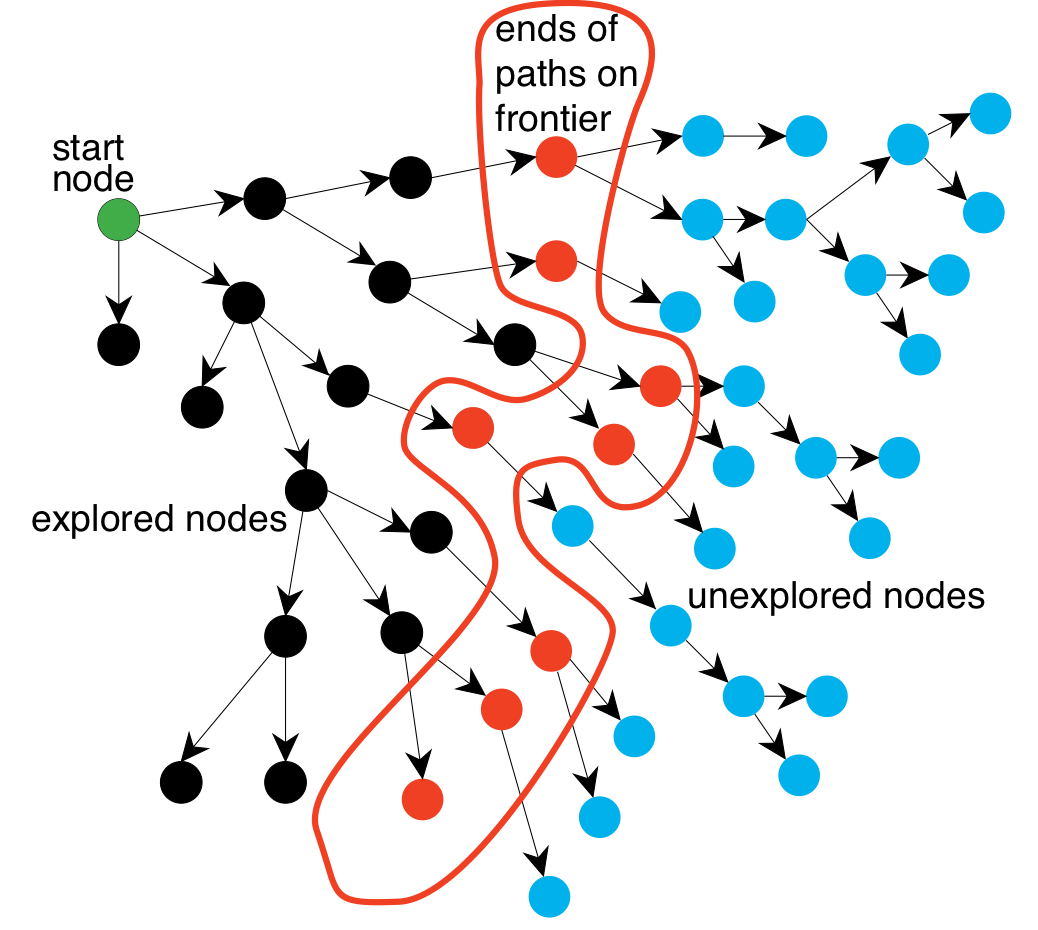
Given a graph, start nodes, and a goal description, incrementally
explore paths from the start nodes. -
Maintain a frontier of nodes that are to be explored.
-
As search proceeds, the frontier expands into the unexplored nodes
until a goal node is encountered. -
The way in which the frontier is expanded defines the search strategy.
-
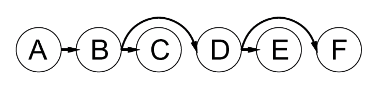
Illustration of searching in a graph
The generic tree search algorithm
- Tree search: Don’t check if nodes are visited multiple times
- function Search(graph, initialState, goalState):
- initialise frontier using the initialState
- while frontier is not empty:
- select and remove node from frontier
- if node.state is a goalState then return node
- for each child in ExpandChildNodes(node, graph):
- add child to frontier if child is not in frontier or exploredSet
- return failure
Using tree search on a graph
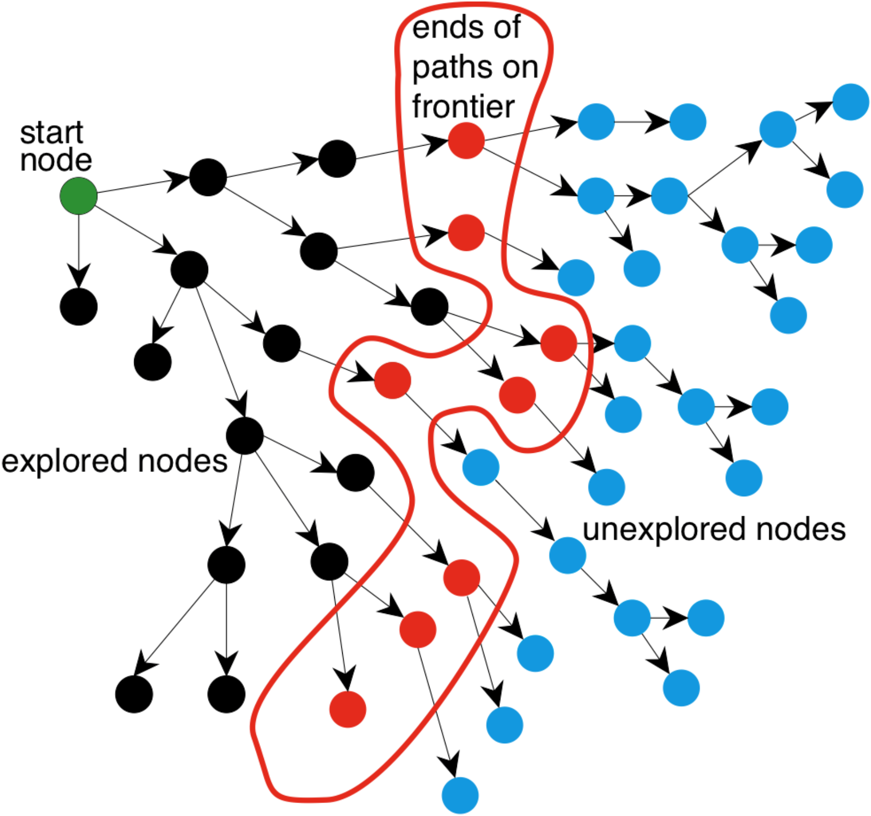
-
- explored nodes might be revisited
- frontier nodes might be duplicated
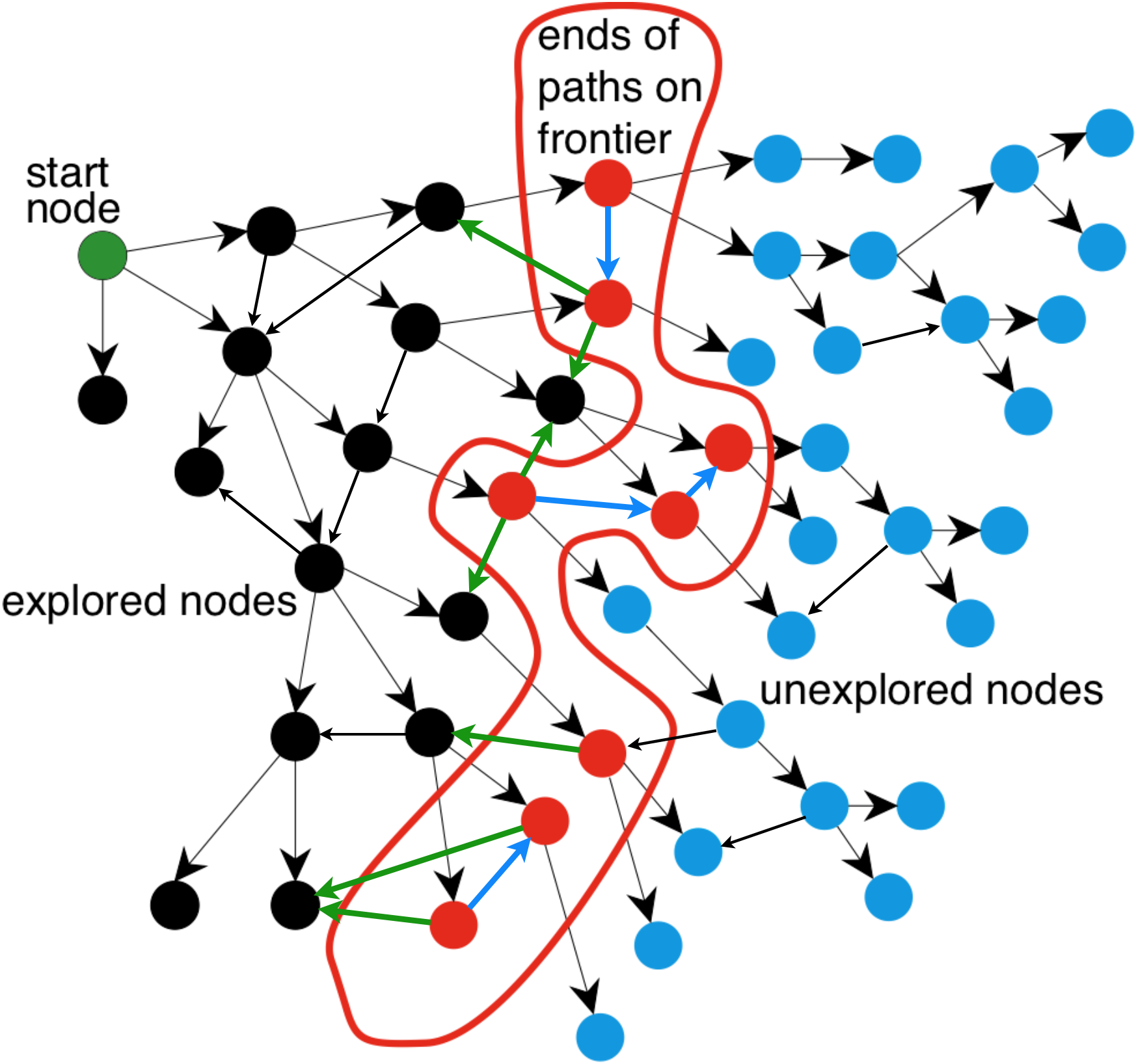
Turning tree search into graph search
- Graph search: Keep track of visited nodes
- function Search(graph, initialState, goalState):
- initialise frontier using the initialState
- initialise exploredSet to the empty set
- while frontier is not empty:
- select and remove node from frontier
- if node.state is a goalState then return node
- add node to exploredSet
- for each child in ExpandChildNodes(node, graph):
- add child to frontier if child is not in frontier or exploredSet
- return failure
Tree search vs. graph search
-
Tree search
- Pro: uses less memory
- Con: might visit the same node several times
-
Graph search
- Pro: only visits nodes at most once
- Con: uses more memory
Depth-first and breadth-first search
These are the two basic search algorithms
- Depth-first search (DFS)
- implement the frontier as a Stack
- space complexity: \( O(bm) \)
- incomplete: might fall into an infinite loop, doesn’t return optimal solution
- Breadth-first search (BFS)
- implement the frontier as a Queue
- space complexity: \( O(b^m) \)
- complete: always finds a solution, if there is one
- (when edge costs are constant, BFS is also optimal)
Iterative deepening
-
Problems with BFS and DFS:
- BFS is guaranteed to halt but uses exponential space.
- DFS uses linear space, but is not guaranteed to halt.
-
Idea: take the best from BFS and DFS — recompute elements of the frontier
rather than saving them.- Look for paths of depth 0, then 1, then 2, then 3, etc.
- Depth-bounded DFS can do this in linear space.
-
Iterative deepening search calls depth-bounded DFS with increasing bounds:
- If a path cannot be found at depth-bound, look for a path at depth-bound + 1.
- Increase depth-bound when the search fails unnaturally
(i.e., if depth-bound was reached).
Iterative deepening complexity
Complexity with solution at depth \(k\) and branching factor \(b\):
| level | # nodes | BFS node visits | ID node visits |
|---|---|---|---|
| \(1\) \(2\) \(3\) \(\vdots\) \(k\) |
\(b\) \(b^{2}\) \(b^{3}\) \(\vdots\) \(b^{k}\) |
\(1\cdot b^{1}\) \(1\cdot b^{2}\) \(1\cdot b^{3}\) \(\vdots\) \(1\cdot b^{k}\) |
\(\,\,\,\,\,\,\,\,k\,\,\cdot b^{1}\) \((k{-}1)\cdot b^{2}\) \((k{-}2)\cdot b^{3}\) \(\,\,\,\,\,\,\,\,\vdots\) \(\,\,\,\,\,\,\,\,1\,\,\cdot b^{k}\) |
| total | \({}\geq b^{k}\) | \({}\leq b^{k}\left(\frac{b}{b-1}\right)^{2}\) |
Numerical comparison for \(k=5\) and \(b=10\):
- BFS = 10 + 100 + 1,000 + 10,000 + 100,000 = 111,110
- IDS = 50 + 400 + 3,000 + 20,000 + 100,000 = 123,450
Note: IDS recalculates shallow nodes several times,
but this doesn’t have a big effect compared to BFS!
Bidirectional search
(will not be in the written examination, but could be used in Shrdlite)
-
Idea: search backward from the goal and forward from the start simultaneously.
-
This can result in an exponential saving, because \(2b^{k/2}\ll b^{k}\).
-
The main problem is making sure the frontiers meet.
-
-
One possible implementation:
-
Use BFS to gradually search backwards from the goal,
building a set of locations that will lead to the goal.- this can be done using dynamic programming
-
Interleave this with forward heuristic search (e.g., A*)
that tries to find a path to these interesting locations.
-
Cost-based search
The frontier is a Priority Queue, ordered by \(f(n)\)
- Uniform-cost search (this is not a heuristic algorithm)
- expand the node with the lowest path cost
- \( f(n) = g(n) \)
- complete and optimal
- Greedy best-first search
- expand the node which is closest to the goal (according to some heuristics)
- \( f(n) = h(n) \)
- incomplete: might fall into an infinite loop, doesn’t return optimal solution
- A* search
- expand the node which has the lowest estimated cost from start to goal
- \( f(n) = g(n) + h(n) \) = estimated cost of the cheapest solution through \(n\)
- complete and optimal (if \(h(n)\) is admissible/consistent)
A* tree search is optimal!
-
A* always finds an optimal solution first, provided that:
-
the branching factor is finite,
-
arc costs are bounded above zero
(i.e., there is some \(\epsilon>0\) such that all
of the arc costs are greater than \(\epsilon\)), and -
\(h(n)\) is admissible
- i.e., \(h(n)\) is nonnegative and an underestimate of
the cost of the shortest path from \(n\) to a goal node.
- i.e., \(h(n)\) is nonnegative and an underestimate of
-
These requirements ensure that \(f\) keeps increasing.
The generic tree search algorithm
Turning tree search into graph search
- Tree search: Don’t check if nodes are visited multiple times
- Graph search: Keep track of visited nodes
- function Search(graph, initialState, goalState):
- initialise frontier using the initialState
- initialise exploredSet to the empty set
- while frontier is not empty:
- select and remove node from frontier
- if node.state is a goalState then return node
- add node to exploredSet
- for each child in ExpandChildNodes(node, graph):
- add child to frontier if child is not in frontier or exploredSet
- return failure
Graph-search = Multiple-path pruning
-
Graph search keeps track of visited nodes, so we don’t visit the same node twice.
-
Suppose that the first time we visit a node is not via the most optimal path
\(\Rightarrow\) then graph search will return a suboptimal path
-
Under which circumstances can we guarantee that A* graph search is optimal?
-
When is A* graph search optimal?
- If \( |h(n’)-h(n)| \leq cost(n’,n) \) for every arc \((n’,n)\),
then A* graph search is optimal: -
- Lemma: the \(f\) values along any path \([…,n’,n,…]\) are nondecreasing:
- Proof: \(g(n) = g(n’) + cost(n’, n)\), therefore:
- \(f(n) = g(n) + h(n) = g(n’) + cost(n’, n) + h(n) \geq g(n’) + h(n’)\)
- therefore: \(f(n) \geq f(n’)\), i.e., \(f\) is nondecreasing
- Lemma: the \(f\) values along any path \([…,n’,n,…]\) are nondecreasing:
-
- Theorem: whenever A* expands a node \(n\), the optimal path to \(n\) has been found
 Proof: Assume this is not true;
- then there must be some \(n’\) still on the frontier, which is on the optimal path to \(n\);
- but \(f(n’) \leq f(n)\);
- and then \(n’\) must already have been expanded \(\Longrightarrow\) contradiction!
- Theorem: whenever A* expands a node \(n\), the optimal path to \(n\) has been found
State-space contours
-
The \(f\) values in A* are nondecreasing, therefore:
first A* expands all nodes with \( f(n) < C \) then A* expands all nodes with \( f(n) = C \) finally A* expands all nodes with \( f(n) > C \) -
A* will not expand any nodes with \( f(n) > C* \),
where \(C*\) is the cost of an optimal solution.
Summary of optimality of A*
-
A* tree search is optimal if:
- the heuristic function \(h(n)\) is admissible
- i.e., \(h(n)\) is nonnegative and an underestimate of the actual cost
- i.e., \( h(n) \leq cost(n,goal) \), for all nodes \(n\)
-
A* graph search is optimal if:
- the heuristic function \(h(n)\) is consistent (or monotone)
- i.e., \( |h(m)-h(n)| \leq cost(m,n) \), for all arcs \((m,n)\)
Summary of tree search strategies
| Search strategy |
Frontier selection |
Halts if solution? | Halts if no solution? | Space usage |
|---|---|---|---|---|
| Depth first | Last node added | No | No | Linear |
| Breadth first | First node added | Yes | No | Exp |
| Greedy best first | Minimal \(h(n)\) | No | No | Exp |
| Uniform cost | Minimal \(g(n)\) | Optimal | No | Exp |
| A* | \(f(n)=g(n)+h(n)\) | Optimal* | No | Exp |
**On finite graphs with cycles, not infinite graphs.
*Provided that \(h(n)\) is admissible.
- Halts if: If there is a path to a goal, it can find one, even on infinite graphs.
- Halts if no: Even if there is no solution, it will halt on a finite graph (with cycles).
- Space: Space complexity as a function of the length of the current path.
Summary of graph search strategies
| Search strategy |
Frontier selection |
Halts if solution? | Halts if no solution? | Space usage |
|---|---|---|---|---|
| Depth first | Last node added | (Yes)** | Yes | Exp |
| Breadth first | First node added | Yes | Yes | Exp |
| Greedy best first | Minimal \(h(n)\) | (Yes)** | Yes | Exp |
| Uniform cost | Minimal \(g(n)\) | Optimal | Yes | Exp |
| A* | \(f(n)=g(n)+h(n)\) | Optimal* | Yes | Exp |
**On finite graphs with cycles, not infinite graphs.
*Provided that \(h(n)\) is consistent.
- Halts if: If there is a path to a goal, it can find one, even on infinite graphs.
- Halts if no: Even if there is no solution, it will halt on a finite graph (with cycles).
- Space: Space complexity as a function of the length of the current path.
Heuristics
Recapitulation: The 8 puzzle
- \(h_{1}(n)\) = number of misplaced tiles
- \(h_{2}(n)\) = total Manhattan distance
(i.e., no. of squares from desired location of each tile)
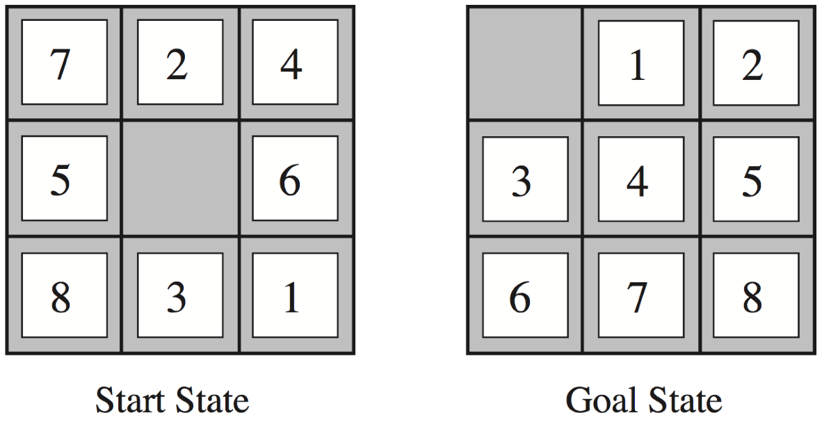
- \(h_{1}(StartState)\) = 8
- \(h_{2}(StartState)\) = 3+1+2+2+2+3+3+2 = 18
Dominating heuristics
-
If (admissible) \(h_{2}(n)\geq h_{1}(n)\) for all \(n\),
then \(h_{2}\) dominates \(h_{1}\) and is better for search. -
Typical search costs (for 8-puzzle):
depth = 14 DFS ≈ 3,000,000 nodes
A*(\(h_1\)) = 539 nodes
A*(\(h_2\)) = 113 nodesdepth = 24 DFS ≈ 54,000,000,000 nodes
A*(\(h_1\)) = 39,135 nodes
A*(\(h_2\)) = 1,641 nodes -
Given any admissible heuristics \(h_{a}\), \(h_{b}\), the maximum heuristics \(h(n)\)
is also admissible and dominates both: \[ h(n) = \max(h_{a}(n),h_{b}(n)) \]
Heuristics from a relaxed problem
-
Admissible heuristics can be derived from the exact solution cost of
a relaxed problem:-
If the rules of the 8-puzzle are relaxed so that a tile can move anywhere,
then \(h_{1}(n)\) gives the shortest solution -
If the rules are relaxed so that a tile can move to any adjacent square,
then \(h_{2}(n)\) gives the shortest solution
-
-
Key point: the optimal solution cost of a relaxed problem is
never greater than the optimal solution cost of the real problem
Non-admissible (non-consistent) A* search
-
A* search with admissible (consistent) heuristics is optimal
-
But what happens if the heuristics is non-admissible?
- i.e., what if \(h(n) > c(n,goal)\), for some \(n\)?
- the solution is not guaranteed to be optimal…
- …but it will find some solution!
-
Why would we want to use a non-admissible heuristics?
- sometimes it’s easier to come up with a heuristics that is almost admissible
- and, often, the search terminates faster!
-
-
* for graph search, \( |h(m)-h(n)| > cost(m,n) \), for some \((m,n)\)
Non-classical search
- A problem is nondeterministic if there are several possible outcomes of an action
- deterministic — nondeterministic (chance)
- It is partially observable if the agent cannot tell exactly which state it is in
- fully observable (perfect info.) — partially observable (imperfect info.)
- A problem can be either nondeterministic, or partially observable, or both:

Nondeterministic search
- We need a more general result function:
- instead of returning a single state, it returns a set of possible outcome states
- e.g., \(\textsf{Results}(\textsf{Suck}, 1) = \{5, 7\}\) and \(\textsf{Results}(\textsf{Suck}, 5) = \{1, 5\}\)
- We also need to generalise the notion of a solution:
- instead of a single sequence (path) from the start to the goal,
we need a strategy (or a contingency plan) - i.e., we need if-then-else constructs
- this is a possible solution from state 1:
- [Suck,
ifState=5then[Right, Suck]else[]]
- [Suck,
- instead of a single sequence (path) from the start to the goal,
How to find contingency plans
(will not be in the written examination)
- We need a new kind of nodes in the search tree:
- and nodes:
these are used whenever an action is nondeterministic - normal nodes are called or nodes:
they are used when we have several possible actions in a state
- and nodes:
- A solution for an and-or search problem is a subtree that:
- has a goal node at every leaf
- specifies exactly one action at each of its or node
- includes every branch at each of its and node
A solution to the erratic vacuum cleaner
(will not be in the written examination)
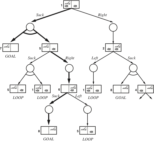
The solution subtree is shown in bold, and corresponds to the plan:
[Suck, if State=5 then [Right, Suck] else []]
Partial observations: Belief states
- Instead of searching in a graph of states, we use belief states
- A belief state is a set of states
- In a sensor-less (or conformant) problem, the agent has no information at all
- The initial belief state is the set of all problem states
- e.g., for the vacuum world the initial state is {1,2,3,4,5,6,7,8}
- The initial belief state is the set of all problem states
- The goal test has to check that all members in the belief state is a goal
- e.g., for the vacuum world, the following are goal states: {7}, {8}, and {7,8}
- The result of performing an action is the union of all possible results
- i.e., \(\textsf{Predict}(b,a) = \{\textsf{Result}(s,a)\) for each \(s\in b\}\)
- if the problem is also nondeterministic:
- \(\textsf{Predict}(b,a) = \bigcup\{\textsf{Results}(s,a)\) for each \(s\in b\}\)
Predicting belief states in the vacuum world
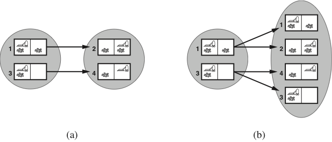
-
(a) Predicting the next belief state for the sensorless vacuum world
with a deterministic action, Right. -
(b) Prediction for the same belief state and action in the nondeterministic
slippery version of the sensorless vacuum world.
Adversarial search (R&N 5.1–5.5)
Types of games
Minimax search
Imperfect decisions
Stochastic games
Games as search problems
-
The main difference to chapters 3–4:
now we have more than one agent that have different goals.-
All possible game sequences are represented in a game tree.
-
The nodes are states of the game, e.g. board positions in chess.
-
Initial state (root) and terminal nodes (leaves).
-
States are connected if there is a legal move/ply.
(a ply is a move by one player, i.e., one layer in the game tree) -
Utility function (payoff function). Terminal nodes have utility values
\({+}x\) (player 1 wins), \({-}x\) (player 2 wins) and \(0\) (draw).
-
Perfect information games: Zero-sum games
-
Perfect information games are solvable in a manner similar to
fully observable single-agent systems, e.g., using forward search. -
If two agents compete, so that a positive reward for one is a negative reward
for the other agent, we have a two-agent zero-sum game. -
The value of a game zero-sum game can be characterized by a single number that one agent is trying to maximize and the other agent is trying to minimize.
-
This leads to a minimax strategy:
- A node is either a MAX node (if it is controlled by the maximising agent),
- or is a MIN node (if it is controlled by the minimising agent).
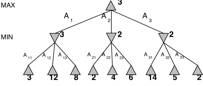
Minimax search
The Minimax algorithm gives perfect play for deterministic, perfect-information games.
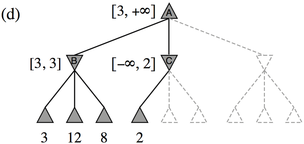
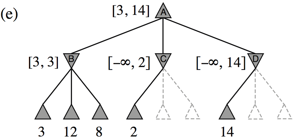
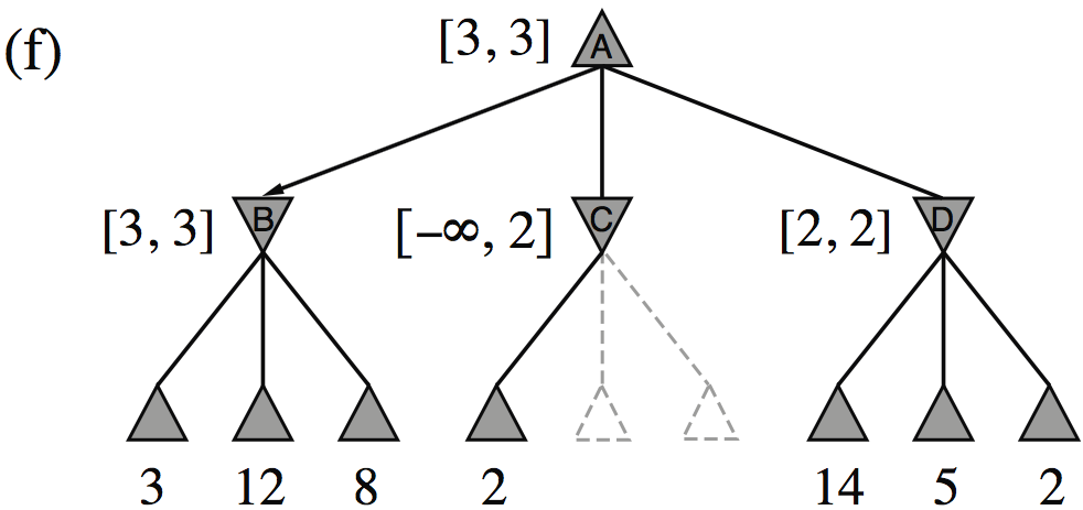
\(\alpha{-}\beta\) pruning
| Minimax(root) | = | \( \max(\min(3,12,8), \min(2,x,y), \min(14,5,2)) \) |
| = | \( \max(3, \min(2,x,y), 2) \) | |
| = | \( \max(3, z, 2) \) where \(z = \min(2,x,y) \leq 2\) | |
| = | \( 3 \) |
- I.e., we don’t need to know the values of \(x\) and \(y\)!
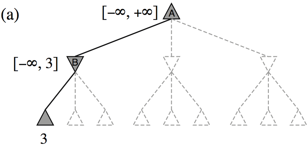
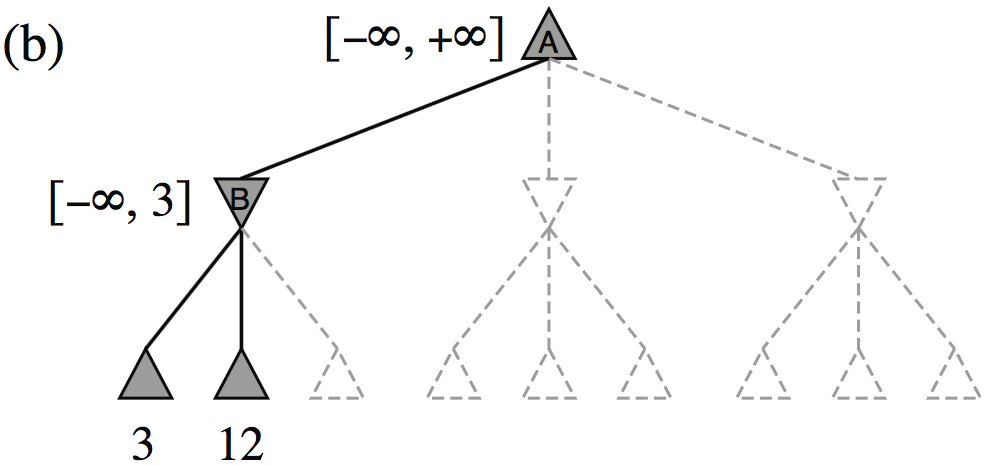
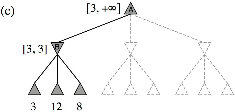
Minimax example, with \(\alpha{-}\beta\) pruning
How efficient is \(\alpha{-}\beta\) pruning?
-
The amount of pruning provided by the α-β algorithm depends on the ordering of the children of each node.
-
It works best if a highest-valued child of a MAX node is selected first and
if a lowest-valued child of a MIN node is returned first. -
In real games, much of the effort is made to optimise the search order.
-
With a “perfect ordering”, the time complexity becomes \(O(b^{m/2})\)
- this doubles the solvable search depth
- however, \(35^{80/2}\) (for chess) or \(250^{160/2}\) (for go) is still quite large…
-
Minimax and real games
-
Most real games are too big to carry out minimax search, even with α-β pruning.
-
For these games, instead of stopping at leaf nodes,
we have to use a cutoff test to decide when to stop. -
The value returned at the node where the algorithm stops
is an estimate of the value for this node. -
The function used to estimate the value is an evaluation function.
-
Much work goes into finding good evaluation functions.
-
There is a trade-off between the amount of computation required
to compute the evaluation function and the size of the search space
that can be explored in any given time.
-
Imperfect decisions
Minimax vs H-minimax
- function Minimax(state):
- if TerminalTest(state) then return Utility(state)
- A := Actions(state)
- if state is a MAX node then return \(\max_{a\in A}\) Minimax(Result(state, a))
- if state is a MIN node then return \(\min_{a\in A}\) Minimax(Result(state, a))
- The Heuristic Minimax algorithm is similar to normal Minimax
- it replaces TerminalTest and Utility with CutoffTest and Eval
- function H-Minimax(state, depth):
- if CutoffTest(state, depth) then return Eval(state)
- A := Actions(state)
- if state is a MAX node then return \(\max_{a\in A}\) H-Minimax(Result(state, a), depth+1)
- if state is a MIN node then return \(\min_{a\in A}\) H-Minimax(Result(state, a), depth+1)
Evaluation functions
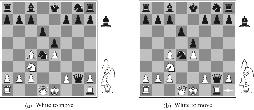
A naive evaluation function will not see the difference between these two states.
\[ Eval(s) = w_1 f_1(s) + w_2 f_2(s) + \cdots + w_n f_n(s) = \sum_{i=1}^{n} w_i f_i(s) \]
Problems with cutoff tests
- Too simplistic cutoff tests and evaluation functions can be problematic:
- e.g., if the cutoff is only based on the current depth
- then it might cut off the search in unfortunate positions
(such as (b) on the previous slide)
- We want more sophisticated cutoff tests:
- only cut off search in quiescent positions
- i.e., in positions that are “stable”, unlikely to exhibit wild swings in value
- non-quiescent positions should be expanded further
Stochastic games
Example: Backgammon
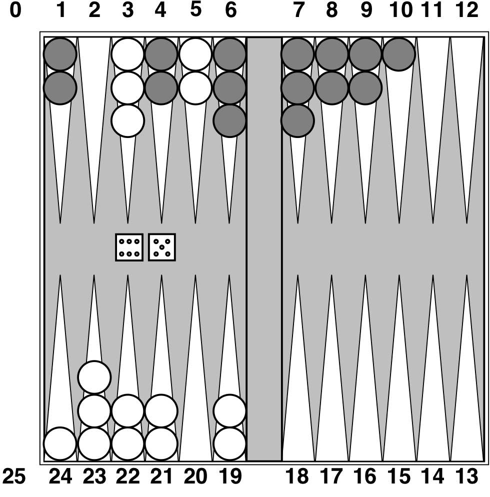
Stochastic games in general
- In stochastic games, chance is introduced by dice, card-shuffling, etc.
- We introduce chance nodes to the game tree.
- We can’t calculate a definite minimax value,
instead we calculate the expected value of a position. - The expected value is the average of all possible outcomes.
- A very simple example with coin-flipping and arbitrary values:
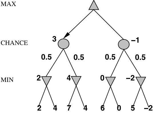
Algorithm for stochastic games
- The ExpectiMinimax algorithm gives perfect play;
- it’s just like Minimax, except we must also handle chance nodes:
- function ExpectiMinimax(state):
- if TerminalTest(state) then return Utility(state)
- A := Actions(state)
- if state is a MAX node then return \(\max_{a\in A}\) ExpectiMinimax(Result(state, a))
- if state is a MAX node then return \(\min_{a\in A}\) ExpectiMinimax(Result(state, a))
- if state is a chance node then return \(\sum_{a\in A}P(a)\)·ExpectiMinimax(Result(state, a))
where \(P(a)\) is the probability that action a occurs.
Constraint satisfaction problems (R&N 4.1, 7.1–7.5)
CSP as a search problem
Improving backtracking efficiency
Constraint propagation
Problem structure
Local search for CSP
CSP: Constraint satisfaction problems
- CSP is a specific kind of search problem:
- the state is defined by variables \(X_{i}\), each taking values from the domain \(D_{i}\)
- the goal test is a set of constraints:
- each constraint specifies allowed values for a subset of variables
- all constraints must be satisfied
- Differences to general search problems:
- the path to a goal isn’t important, only the solution is.
- there are no predefined starting state
- often these problems are huge, with thousands of variables,
so systematically searching the space is infeasible
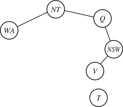
Example: Map colouring (binary CSP)
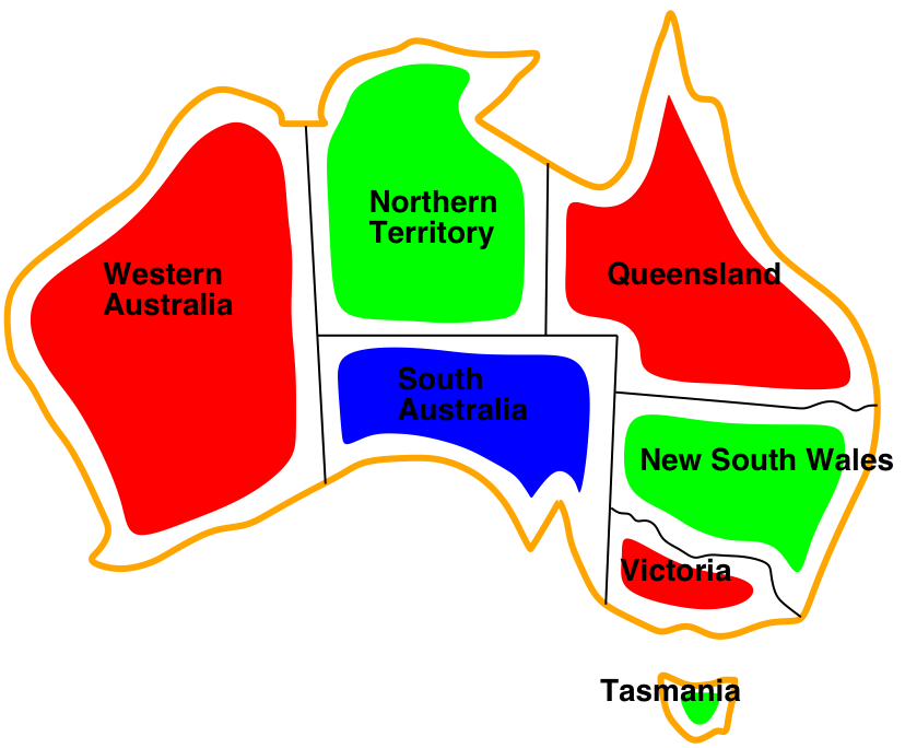
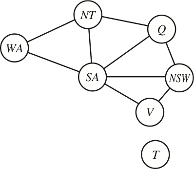
| Variables: | WA, NT, Q, NSW, V, SA, T |
| Domains: | \(D_i\) = {red, green, blue} |
| Constraints: | SA≠WA, SA≠NT, SA≠Q, SA≠NSW, SA≠V, WA≠NT, NT≠Q, Q≠NSW, NSW≠V |
| Constraint graph: | Every variable is a node, every binary constraint is an arc. |
Example: Cryptarithmetic puzzle (higher-order CSP)
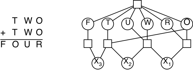
| Variables: | F, T, U, W, R, O, \(X_1, X_2, X_3\) |
| Domains: | \(D_i\) = {0, 1, 2, 3, 4, 5, 6, 7, 8, 9} |
| Constraints: | Alldiff(F,T,U,W,R,O), O+O=R+10·\(X_1\), etc. |
| Constraint graph: | This is not a binary CSP! The graph is a constraint hypergraph. |
Algorithm for backtracking search
- At each depth level, decide on one single variable to assign:
- this gives branching factor \(b=d\), so there are \(d^{n}\) leaves
- Depth-first search with single-variable assignments is called backtracking search:
- function BacktrackingSearch(csp):
- return Backtrack(csp, { })
- function Backtrack(csp, assignment):
- if assignment is complete then return assignment
- var := SelectUnassignedVariable(csp, assignment)
- for each value in OrderDomainValues(csp, var, assignment):
- if value is consistent with assignment:
- inferences := Inference(csp, var, value)
- if inferences ≠ failure:
- result := Backtrack(csp, assignment \(\cup\) {var=value} \(\cup\) inferences)
- if result ≠ failure then return result
- if value is consistent with assignment:
- return failure
Improving backtracking efficiency
-
The general-purpose algorithm gives rise to several questions:
- Which variable should be assigned next?
- SelectUnassignedVariable(csp, assignment)
- In what order should its values be tried?
- OrderDomainValues(csp, var, assignment)
- What inferences should be performed at each step?
- Inference(csp, var, value)
- Which variable should be assigned next?
Selecting unassigned variables
-
Heuristics for selecting the next unassigned variable:
-
Minimum remaining values (MRV):
\(\Longrightarrow\) choose the variable with the fewest legal values
-
Degree heuristic (if there are several MRV variables):
\(\Longrightarrow\) choose the variable with most constraints on remaining variables
-
Ordering domain values
-
Heuristics for ordering the values of a selected variable:
- Least constraining value:
\(\Longrightarrow\) prefer the value that rules out the fewest choices
for the neighboring variables in the constraint graph
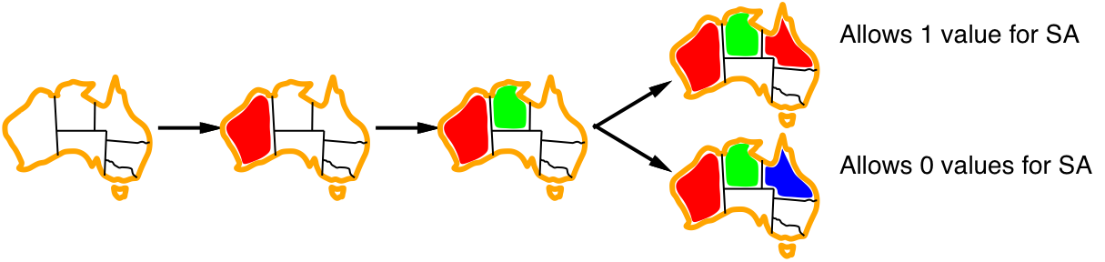
- Least constraining value:
Constraint propagation
Inference: Arc consistency, AC-3
- Keep a set of arcs to be considered: pick one arc \((X,Y)\) at the time and
make it consistent (i.e., make \(X\) arc consistent to \(Y\)).
- Start with the set of all arcs \(\{(X,Y),(Y,X),(X,Z),(Z,X),\ldots\}\).
- When an arc has been made arc consistent, does it ever need to be checked again?
- An arc \((Z,X)\) needs to be revisited if the domain of \(X\) is revised.
- function AC-3(inout csp):
- initialise queue to all arcs in csp
- while queue is not empty:
- (X, Y) := RemoveOne(queue)
- if Revise(csp, X, Y):
- if \(D_X=\emptyset\) then return failure
- for each Z in X.neighbors–{Y} do add (Z, X) to queue
- function Revise(inout csp, X, Y):
- delete every x from \(D_X\) such that there is no value y in \(D_Y\) satisfying the constraint \(C_{XY}\)
- return true if \(D_X\) was revised
Combining backtracking with AC-3
-
What if some domains have more than one element after AC?
-
We can resort to backtracking search:
- Select a variable and a value using some heuristics
(e.g., minimum-remaining-values, degree-heuristic, least-constraining-value) - Make the graph arc-consistent again
- Backtrack and try new values/variables, if AC fails
- Select a new variable/value, perform arc-consistency, etc.
- Select a variable and a value using some heuristics
-
Do we need to restart AC from scratch?
- no, only some arcs risk becoming inconsistent after a new assignment
- restart AC with the queue \(\{(Y_i,X) | X\rightarrow Y_i\}\),
i.e., only the arcs \((Y_i,X)\) where \(Y_i\) are the neighbors of \(X\) - this algorithm is called Maintaining Arc Consistency (MAC)
Consistency properties
-
There are several kinds of consistency properties and algorithms:
-
Node consistency: single variable, unary constraints (straightforward)
-
Arc consistency: pairs of variables, binary constraints (AC-3 algorithm)
-
Path consistency: triples of variables, binary constraints (PC-2 algorithm)
-
\(k\)-consistency: \(k\) variables, \(k\)-ary constraints (algorithms exponential in \(k\))
-
Consistency for global constraints:
Special-purpose algorithms for different constraints, e.g.:- Alldiff(\(X_1,\ldots,X_m\)) is inconsistent if \(m > |D_1\cup\cdots\cup D_m|\)
- Atmost(\(n,X_1,\ldots,X_m\)) is inconsistent if \(n < \sum_i \min(D_i)\)
-
Problem structure
Tree-structured CSP
(will not be in the written examination)
- A constraint graph is a tree when any two variables are connected by only one path.
- then any variable can act as root in the tree
- tree-structured CSP can be solved in linear time, in the number of variables!
- To solve a tree-structured CSP:
- first pick a variable to be the root of the tree
- then find a topological sort of the variables (with the root first)
- finally, make each arc consistent, in reverse topological order
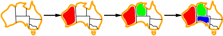
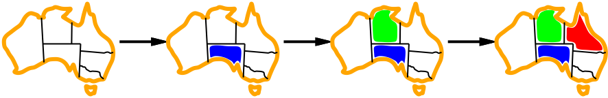
Converting to tree-structured CSP
(will not be in the written examination)
- Most CSPs are not tree-structured, but sometimes we can reduce them to a tree
- one approach is to assign values to some variables,
so that the remaining variables form a tree
- one approach is to assign values to some variables,
-
If we assign a colour to South Australia, then the remaining variables form a tree
- An alternative is to assign values to {NT,Q,V}: But this is worse than assigning South Australia, because then we have to try 3×3×3 different assignments, and for each of them solve the remaining tree-CSP
Local search for CSP
- Given an assignment of a value to each variable:
- A conflict is an unsatisfied constraint.
- The goal is an assignment with zero conflicts.
- Heuristic function to be minimized: the number of conflicts.
- this is the min-conflicts heuristics
- function MinConflicts(csp, max_steps)
- current := an initial complete assignment for csp
- repeat max_steps times:
- if current is a solution for csp then return current
- var := a randomly chosen conflicted variable from csp
- value := the value v for var that minimises Conflicts(var, v, current, csp)
- current[var] = value
- return failure
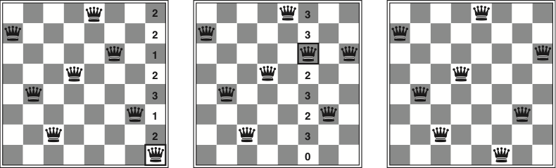
Example: \(n\)-queens (revisited)
- Put \(n\) queens on an \(n\times n\) board, in separate columns
- Conflicts = unsatisfied constraints = n:o of threatened queens
- Move a queen to reduce the number of conflicts
- repeat until we cannot move any queen anymore
- then we are at a local maximum — hopefully it is global too
Example: Travelling salesperson
-
Start with any complete tour, and perform pairwise exchanges
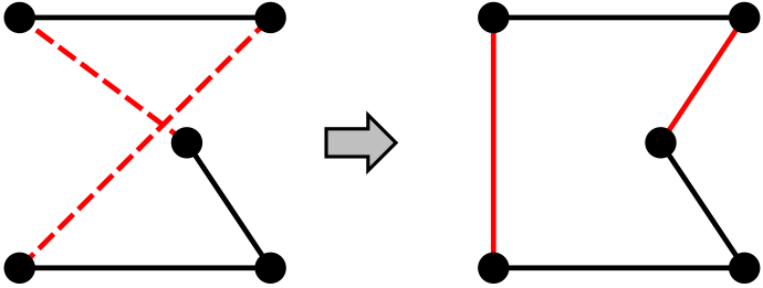
-
Variants of this approach get within 1% of optimal
very quickly with thousands of cities
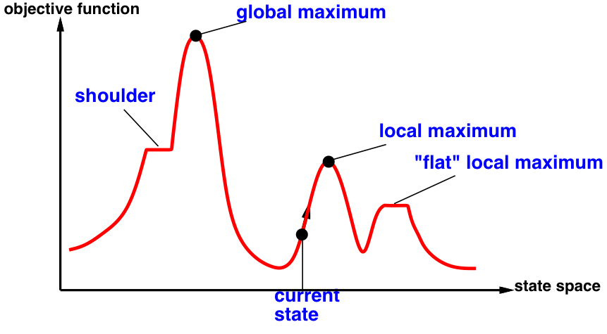
Local search
Hill climbing search is also called gradient/steepest ascent/descent,
or greedy local search.
- function HillClimbing(graph, initialState):
- current := initialState
- loop:
- neighbor := a highest-valued successor of current
- if neighbor.value ≤ current.value then return current
- current := neighbor
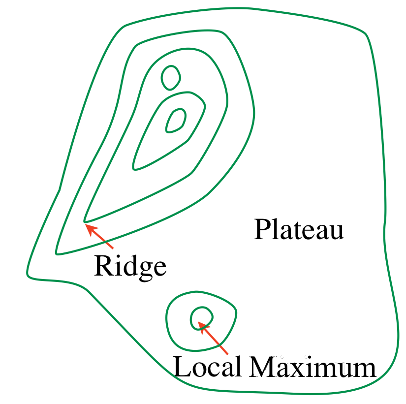
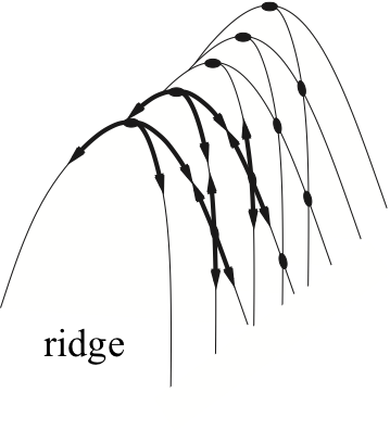
Problems with hill climbing
Local maxima — Ridges — Plateaux
Randomized hill climbing
-
As well as upward steps we can allow for:
-
Random steps: (sometimes) move to a random neighbor.
-
Random restart: (sometimes) reassign random values to all variables.
-
-
Both variants can be combined!
1-dimensional illustrative example
-
Two 1-dimensional search spaces; you can step right or left:
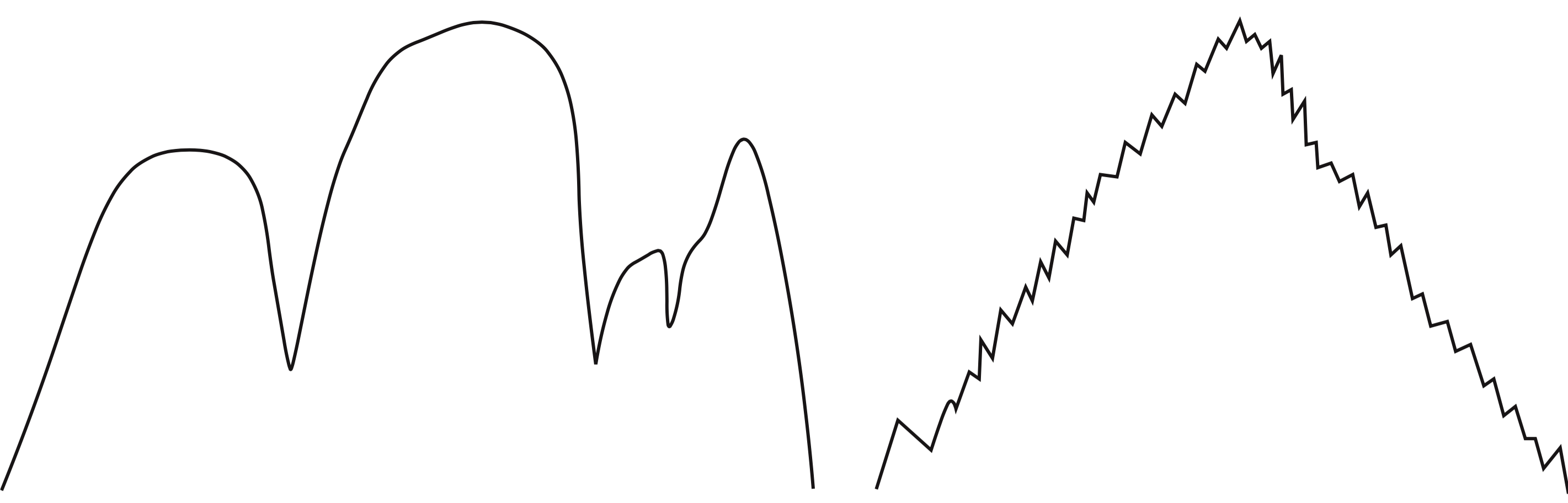
- Which method would most easily find the global maximum?
- random steps or random restarts?
- What if we have hundreds or thousands of dimensions?
- …where different dimensions have different structure?